SQL – Overview
SQL is a language to operate databases; it includes database creation, deletion, fetching rows, modifying rows, etc. SQL is an ANSI (American National Standards Institute) standard language, but there are many different versions of the SQL language.
What is SQL?
SQL is Structured Query Language, which is a computer language for storing, manipulating and retrieving data stored in a relational database.
SQL is the standard language for Relational Database System. All the Relational Database Management Systems (RDMS) like MySQL, MS Access, Oracle, Sybase, Informix, Postgres and SQL Server use SQL as their standard database language.
Also, they are using different dialects, such as −
- MS SQL Server using T-SQL,
- Oracle using PL/SQL,
- MS Access version of SQL is called JET SQL (native format) etc.
Why SQL?
SQL is widely popular because it offers the following advantages −
-
Allows users to access data in the relational database management systems.
-
Allows users to describe the data.
-
Allows users to define the data in a database and manipulate that data.
-
Allows to embed within other languages using SQL modules, libraries & pre-compilers.
-
Allows users to create and drop databases and tables.
-
Allows users to create view, stored procedure, functions in a database.
-
Allows users to set permissions on tables, procedures and views.
A Brief History of SQL
-
1970 − Dr. Edgar F. “Ted” Codd of IBM is known as the father of relational databases. He described a relational model for databases.
-
1974 − Structured Query Language appeared.
-
1978 − IBM worked to develop Codd”s ideas and released a product named System/R.
-
1986 − IBM developed the first prototype of relational database and standardized by ANSI. The first relational database was released by Relational Software which later came to be known as Oracle.
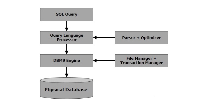
SQL Process
When you are executing an SQL command for any RDBMS, the system determines the best way to carry out your request and SQL engine figures out how to interpret the task.
There are various components included in this process.
These components are −
- Query Dispatcher
- Optimization Engines
- Classic Query Engine
- SQL Query Engine, etc.
A classic query engine handles all the non-SQL queries, but a SQL query engine won”t handle logical files.
Following is a simple diagram showing the SQL Architecture −
SQL Commands
The standard SQL commands to interact with relational databases are CREATE, SELECT, INSERT, UPDATE, DELETE and DROP. These commands can be classified into the following groups based on their nature −
DDL – Data Definition Language
| Sr.No. |
Command & Description |
| 1 |
CREATE
Creates a new table, a view of a table, or other object in the database.
|
| 2 |
ALTER
Modifies an existing database object, such as a table.
|
| 3 |
DROP
Deletes an entire table, a view of a table or other objects in the database.
|
DML – Data Manipulation Language
| Sr.No. |
Command & Description |
| 1 |
SELECT
Retrieves certain records from one or more tables.
|
| 2 |
INSERT
Creates a record.
|
| 3 |
UPDATE
Modifies records.
|
| 4 |
DELETE
Deletes records.
|
DCL – Data Control Language
| Sr.No. |
Command & Description |
| 1 |
GRANT
Gives a privilege to user.
|
| 2 |
REVOKE
Takes back privileges granted from user.
|
SQL – RDBMS Concepts
What is RDBMS?
RDBMS stands for Relational Database Management System. RDBMS is the basis for SQL, and for all modern database systems like MS SQL Server, IBM DB2, Oracle, MySQL, and Microsoft Access.
A Relational database management system (RDBMS) is a database management system (DBMS) that is based on the relational model as introduced by E. F. Codd.
What is a table?
The data in an RDBMS is stored in database objects which are called as tables. This table is basically a collection of related data entries and it consists of numerous columns and rows.
Remember, a table is the most common and simplest form of data storage in a relational database. The following program is an example of a CUSTOMERS table −
+----+----------+-----+-----------+----------+
| ID | NAME     | AGE | ADDRESS   | SALARY   |
+----+----------+-----+-----------+----------+
|  1 | Ramesh   |  32 | Ahmedabad |  2000.00 |
|  2 | Khilan   |  25 | Delhi     |  1500.00 |
|  3 | kaushik  |  23 | Kota      |  2000.00 |
|  4 | Chaitali |  25 | Mumbai    |  6500.00 |
|  5 | Hardik   |  27 | Bhopal    |  8500.00 |
|  6 | Komal    |  22 | MP        |  4500.00 |
|  7 | Muffy    |  24 | Indore    | 10000.00 |
+----+----------+-----+-----------+----------+
What is a field?
Every table is broken up into smaller entities called fields. The fields in the CUSTOMERS table consist of ID, NAME, AGE, ADDRESS and SALARY.
A field is a column in a table that is designed to maintain specific information about every record in the table.
What is a Record or a Row?
A record is also called as a row of data is each individual entry that exists in a table. For example, there are 7 records in the above CUSTOMERS table. Following is a single row of data or record in the CUSTOMERS table −
+----+----------+-----+-----------+----------+
|  1 | Ramesh   |  32 | Ahmedabad |  2000.00 |
+----+----------+-----+-----------+----------+
A record is a horizontal entity in a table.
What is a column?
A column is a vertical entity in a table that contains all information associated with a specific field in a table.
For example, a column in the CUSTOMERS table is ADDRESS, which represents location description and would be as shown below −
+-----------+
| ADDRESS   |
+-----------+
| Ahmedabad |
| Delhi     |
| Kota      |
| Mumbai    |
| Bhopal    |
| MP        |
| Indore    |
+----+------+
What is a NULL value?
A NULL value in a table is a value in a field that appears to be blank, which means a field with a NULL value is a field with no value.
It is very important to understand that a NULL value is different than a zero value or a field that contains spaces. A field with a NULL value is the one that has been left blank during a record creation.
SQL Constraints
Constraints are the rules enforced on data columns on a table. These are used to limit the type of data that can go into a table. This ensures the accuracy and reliability of the data in the database.
Constraints can either be column level or table level. Column level constraints are applied only to one column whereas, table level constraints are applied to the entire table.
Following are some of the most commonly used constraints available in SQL −
-
− Ensures that a column cannot have a NULL value.
-
− Ensures that all the values in a column are different.
-
− Uniquely identifies each row/record in a database table.
-
− Uniquely identifies a row/record in any another database table.
-
− Used to create and retrieve data from the database very quickly.
Data Integrity
The following categories of data integrity exist with each RDBMS −
-
Entity Integrity − There are no duplicate rows in a table.
-
Domain Integrity − Enforces valid entries for a given column by restricting the type, the format, or the range of values.
-
Referential integrity − Rows cannot be deleted, which are used by other records.
-
User-Defined Integrity − Enforces some specific business rules that do not fall into entity, domain or referential integrity.
Database Normalization
Database normalization is the process of efficiently organizing data in a database. There are two reasons of this normalization process −
-
Eliminating redundant data, for example, storing the same data in more than one table.
-
Ensuring data dependencies make sense.
Both these reasons are worthy goals as they reduce the amount of space a database consumes and ensures that data is logically stored. Normalization consists of a series of guidelines that help guide you in creating a good database structure.
Normalization guidelines are divided into normal forms; think of a form as the format or the way a database structure is laid out. The aim of normal forms is to organize the database structure, so that it complies with the rules of first normal form, then second normal form and finally the third normal form.
It is your choice to take it further and go to the fourth normal form, fifth normal form and so on, but in general, the third normal form is more than enough.
SQL – RDBMS Databases
There are many popular RDBMS available to work with. This tutorial gives a brief overview of some of the most popular RDBMSâs. This would help you to compare their basic features.
MySQL
MySQL is an open source SQL database, which is developed by a Swedish company â MySQL AB. MySQL is pronounced as “my ess-que-ell,” in contrast with SQL, pronounced “sequel.”
MySQL is supporting many different platforms including Microsoft Windows, the major Linux distributions, UNIX, and Mac OS X.
MySQL has free and paid versions, depending on its usage (non-commercial/commercial) and features. MySQL comes with a very fast, multi-threaded, multi-user and robust SQL database server.
History
-
Development of MySQL by Michael Widenius & David Axmark beginning in 1994.
-
First internal release on 23rd May 1995.
-
Windows Version was released on the 8th January 1998 for Windows 95 and NT.
-
Version 3.23: beta from June 2000, production release January 2001.
-
Version 4.0: beta from August 2002, production release March 2003 (unions).
-
Version 4.1: beta from June 2004, production release October 2004.
-
Version 5.0: beta from March 2005, production release October 2005.
-
Sun Microsystems acquired MySQL AB on the 26th February 2008.
-
Version 5.1: production release 27th November 2008.
Features
- High Performance.
- High Availability.
- Scalability and Flexibility Run anything.
- Robust Transactional Support.
- Web and Data Warehouse Strengths.
- Strong Data Protection.
- Comprehensive Application Development.
- Management Ease.
- Open Source Freedom and 24 x 7 Support.
- Lowest Total Cost of Ownership.
MS SQL Server
MS SQL Server is a Relational Database Management System developed by Microsoft Inc. Its primary query languages are −
History
-
1987 – Sybase releases SQL Server for UNIX.
-
1988 – Microsoft, Sybase, and Aston-Tate port SQL Server to OS/2.
-
1989 – Microsoft, Sybase, and Aston-Tate release SQL Server 1.0 for OS/2.
-
1990 – SQL Server 1.1 is released with support for Windows 3.0 clients.
-
Aston – Tate drops out of SQL Server development.
-
2000 – Microsoft releases SQL Server 2000.
-
2001 – Microsoft releases XML for SQL Server Web Release 1 (download).
-
2002 – Microsoft releases SQLXML 2.0 (renamed from XML for SQL Server).
-
2002 – Microsoft releases SQLXML 3.0.
-
2005 – Microsoft releases SQL Server 2005 on November 7th, 2005.
Features
- High Performance
- High Availability
- Database mirroring
- Database snapshots
- CLR integration
- Service Broker
- DDL triggers
- Ranking functions
- Row version-based isolation levels
- XML integration
- TRY…CATCH
- Database Mail
ORACLE
It is a very large multi-user based database management system. Oracle is a relational database management system developed by ”Oracle Corporation”.
Oracle works to efficiently manage its resources, a database of information among the multiple clients requesting and sending data in the network.
It is an excellent database server choice for client/server computing. Oracle supports all major operating systems for both clients and servers, including MSDOS, NetWare, UnixWare, OS/2 and most UNIX flavors.
History
Oracle began in 1977 and celebrating its 32 wonderful years in the industry (from 1977 to 2009).
-
1977 – Larry Ellison, Bob Miner and Ed Oates founded Software Development Laboratories to undertake development work.
-
1979 – Version 2.0 of Oracle was released and it became first commercial relational database and first SQL database. The company changed its name to Relational Software Inc. (RSI).
-
1981 – RSI started developing tools for Oracle.
-
1982 – RSI was renamed to Oracle Corporation.
-
1983 – Oracle released version 3.0, rewritten in C language and ran on multiple platforms.
-
1984 – Oracle version 4.0 was released. It contained features like concurrency control – multi-version read consistency, etc.
-
1985 – Oracle version 4.0 was released. It contained features like concurrency control – multi-version read consistency, etc.
-
2007 – Oracle released Oracle11g. The new version focused on better partitioning, easy migration, etc.
Features
- Concurrency
- Read Consistency
- Locking Mechanisms
- Quiesce Database
- Portability
- Self-managing database
- SQL*Plus
- ASM
- Scheduler
- Resource Manager
- Data Warehousing
- Materialized views
- Bitmap indexes
- Table compression
- Parallel Execution
- Analytic SQL
- Data mining
- Partitioning
MS ACCESS
This is one of the most popular Microsoft products. Microsoft Access is an entry-level database management software. MS Access database is not only inexpensive but also a powerful database for small-scale projects.
MS Access uses the Jet database engine, which utilizes a specific SQL language dialect (sometimes referred to as Jet SQL).
MS Access comes with the professional edition of MS Office package. MS Access has easyto-use intuitive graphical interface.
-
1992 – Access version 1.0 was released.
-
1993 – Access 1.1 released to improve compatibility with inclusion the Access Basic programming language.
-
The most significant transition was from Access 97 to Access 2000.
-
2007 – Access 2007, a new database format was introduced ACCDB which supports complex data types such as multi valued and attachment fields.
Features
-
Users can create tables, queries, forms and reports and connect them together with macros.
-
Option of importing and exporting the data to many formats including Excel, Outlook, ASCII, dBase, Paradox, FoxPro, SQL Server, Oracle, ODBC, etc.
-
There is also the Jet Database format (MDB or ACCDB in Access 2007), which can contain the application and data in one file. This makes it very convenient to distribute the entire application to another user, who can run it in disconnected environments.
-
Microsoft Access offers parameterized queries. These queries and Access tables can be referenced from other programs like VB6 and .NET through DAO or ADO.
-
The desktop editions of Microsoft SQL Server can be used with Access as an alternative to the Jet Database Engine.
-
Microsoft Access is a file server-based database. Unlike the client-server relational database management systems (RDBMS), Microsoft Access does not implement database triggers, stored procedures or transaction logging.
SQL – Syntax
SQL is followed by a unique set of rules and guidelines called Syntax. This tutorial gives you a quick start with SQL by listing all the basic SQL Syntax.
All the SQL statements start with any of the keywords like SELECT, INSERT, UPDATE, DELETE, ALTER, DROP, CREATE, USE, SHOW and all the statements end with a semicolon (;).
The most important point to be noted here is that SQL is case insensitive, which means SELECT and select have same meaning in SQL statements. Whereas, MySQL makes difference in table names. So, if you are working with MySQL, then you need to give table names as they exist in the database.
Various Syntax in SQL
All the examples given in this tutorial have been tested with a MySQL server.
SQL SELECT Statement
SELECT column1, column2....columnN
FROM   table_name;
SQL DISTINCT Clause
SELECT DISTINCT column1, column2....columnN
FROM   table_name;
SQL WHERE Clause
SELECT column1, column2....columnN
FROM   table_name
WHERE  CONDITION;
SQL AND/OR Clause
SELECT column1, column2....columnN
FROM   table_name
WHERE  CONDITION-1 {AND|OR} CONDITION-2;
SQL IN Clause
SELECT column1, column2....columnN
FROM   table_name
WHERE  column_name IN (val-1, val-2,...val-N);
SQL BETWEEN Clause
SELECT column1, column2....columnN
FROM   table_name
WHERE  column_name BETWEEN val-1 AND val-2;
SQL LIKE Clause
SELECT column1, column2....columnN
FROM   table_name
WHERE  column_name LIKE { PATTERN };
SQL ORDER BY Clause
SELECT column1, column2....columnN
FROM   table_name
WHERE  CONDITION
ORDER BY column_name {ASC|DESC};
SQL GROUP BY Clause
SELECT SUM(column_name)
FROM   table_name
WHERE  CONDITION
GROUP BY column_name;
SQL COUNT Clause
SELECT COUNT(column_name)
FROM   table_name
WHERE  CONDITION;
SQL HAVING Clause
SELECT SUM(column_name)
FROM   table_name
WHERE  CONDITION
GROUP BY column_name
HAVING (arithematic function condition);
SQL CREATE TABLE Statement
CREATE TABLE table_name(
column1 datatype,
column2 datatype,
column3 datatype,
.....
columnN datatype,
PRIMARY KEY( one or more columns )
);
SQL DROP TABLE Statement
DROP TABLE table_name;
SQL CREATE INDEX Statement
CREATE UNIQUE INDEX index_name
ON table_name ( column1, column2,...columnN);
SQL DROP INDEX Statement
ALTER TABLE table_name
DROP INDEX index_name;
SQL DESC Statement
DESC table_name;
SQL TRUNCATE TABLE Statement
TRUNCATE TABLE table_name;
SQL ALTER TABLE Statement
ALTER TABLE table_name {ADD|DROP|MODIFY} column_name {data_ype};
SQL ALTER TABLE Statement (Rename)
ALTER TABLE table_name RENAME TO new_table_name;
SQL INSERT INTO Statement
INSERT INTO table_name( column1, column2....columnN)
VALUES ( value1, value2....valueN);
SQL UPDATE Statement
UPDATE table_name
SET column1 = value1, column2 = value2....columnN=valueN
[ WHERE  CONDITION ];
SQL DELETE Statement
DELETE FROM table_name
WHERE  {CONDITION};
SQL CREATE DATABASE Statement
CREATE DATABASE database_name;
SQL DROP DATABASE Statement
DROP DATABASE database_name;
SQL USE Statement
USE database_name;
SQL COMMIT Statement
COMMIT;
SQL ROLLBACK Statement
ROLLBACK;
SQL – Data Types
SQL Data Type is an attribute that specifies the type of data of any object. Each column, variable and expression has a related data type in SQL. You can use these data types while creating your tables. You can choose a data type for a table column based on your requirement.
SQL Server offers six categories of data types for your use which are listed below −
Exact Numeric Data Types
| DATA TYPE |
FROM |
TO |
| bigint |
-9,223,372,036,854,775,808 |
9,223,372,036,854,775,807 |
| int |
-2,147,483,648 |
2,147,483,647 |
| smallint |
-32,768 |
32,767 |
| tinyint |
0 |
255 |
| bit |
0 |
1 |
| decimal |
-10^38 +1 |
10^38 -1 |
| numeric |
-10^38 +1 |
10^38 -1 |
| money |
-922,337,203,685,477.5808 |
+922,337,203,685,477.5807 |
| smallmoney |
-214,748.3648 |
+214,748.3647 |
Approximate Numeric Data Types
| DATA TYPE |
FROM |
TO |
| float |
-1.79E + 308 |
1.79E + 308 |
| real |
-3.40E + 38 |
3.40E + 38 |
Date and Time Data Types
| DATA TYPE |
FROM |
TO |
| datetime |
Jan 1, 1753 |
Dec 31, 9999 |
| smalldatetime |
Jan 1, 1900 |
Jun 6, 2079 |
| date |
Stores a date like June 30, 1991 |
| time |
Stores a time of day like 12:30 P.M. |
Note − Here, datetime has 3.33 milliseconds accuracy where as smalldatetime has 1 minute accuracy.
Character Strings Data Types
| Sr.No. |
DATA TYPE & Description |
| 1 |
char
Maximum length of 8,000 characters.( Fixed length non-Unicode characters)
|
| 2 |
varchar
Maximum of 8,000 characters.(Variable-length non-Unicode data).
|
| 3 |
varchar(max)
Maximum length of 2E + 31 characters, Variable-length non-Unicode data (SQL Server 2005 only).
|
| 4 |
text
Variable-length non-Unicode data with a maximum length of 2,147,483,647 characters.
|
Unicode Character Strings Data Types
| Sr.No. |
DATA TYPE & Description |
| 1 |
nchar
Maximum length of 4,000 characters.( Fixed length Unicode)
|
| 2 |
nvarchar
Maximum length of 4,000 characters.(Variable length Unicode)
|
| 3 |
nvarchar(max)
Maximum length of 2E + 31 characters (SQL Server 2005 only).( Variable length Unicode)
|
| 4 |
ntext
Maximum length of 1,073,741,823 characters. ( Variable length Unicode )
|
Binary Data Types
| Sr.No. |
DATA TYPE & Description |
| 1 |
binary
Maximum length of 8,000 bytes(Fixed-length binary data )
|
| 2 |
varbinary
Maximum length of 8,000 bytes.(Variable length binary data)
|
| 3 |
varbinary(max)
Maximum length of 2E + 31 bytes (SQL Server 2005 only). ( Variable length Binary data)
|
| 4 |
image
Maximum length of 2,147,483,647 bytes. ( Variable length Binary Data)
|
Misc Data Types
| Sr.No. |
DATA TYPE & Description |
| 1 |
sql_variant
Stores values of various SQL Server-supported data types, except text, ntext, and timestamp.
|
| 2 |
timestamp
Stores a database-wide unique number that gets updated every time a row gets updated
|
| 3 |
uniqueidentifier
Stores a globally unique identifier (GUID)
|
| 4 |
xml
Stores XML data. You can store xml instances in a column or a variable (SQL Server 2005 only).
|
| 5 |
cursor
Reference to a cursor object
|
| 6 |
table
Stores a result set for later processing
|
SQL – Operators
What is an Operator in SQL?
An operator is a reserved word or a character used primarily in an SQL statement”s WHERE clause to perform operation(s), such as comparisons and arithmetic operations. These Operators are used to specify conditions in an SQL statement and to serve as conjunctions for multiple conditions in a statement.
- Arithmetic operators
- Comparison operators
- Logical operators
- Operators used to negate conditions
SQL Arithmetic Operators
Assume ”variable a” holds 10 and ”variable b” holds 20, then −
| Operator |
Description |
Example |
| + (Addition) |
Adds values on either side of the operator. |
a + b will give 30 |
| – (Subtraction) |
Subtracts right hand operand from left hand operand. |
a – b will give -10 |
| * (Multiplication) |
Multiplies values on either side of the operator. |
a * b will give 200 |
| / (Division) |
Divides left hand operand by right hand operand. |
b / a will give 2 |
| % (Modulus) |
Divides left hand operand by right hand operand and returns remainder. |
b % a will give 0 |
SQL Comparison Operators
Assume ”variable a” holds 10 and ”variable b” holds 20, then −
| Operator |
Description |
Example |
| = |
Checks if the values of two operands are equal or not, if yes then condition becomes true. |
(a = b) is not true. |
| != |
Checks if the values of two operands are equal or not, if values are not equal then condition becomes true. |
(a != b) is true. |
| <> |
Checks if the values of two operands are equal or not, if values are not equal then condition becomes true. |
(a <> b) is true. |
| > |
Checks if the value of left operand is greater than the value of right operand, if yes then condition becomes true. |
(a > b) is not true. |
| < |
Checks if the value of left operand is less than the value of right operand, if yes then condition becomes true. |
(a < b) is true. |
| >= |
Checks if the value of left operand is greater than or equal to the value of right operand, if yes then condition becomes true. |
(a >= b) is not true. |
| <= |
Checks if the value of left operand is less than or equal to the value of right operand, if yes then condition becomes true. |
(a <= b) is true. |
| !< |
Checks if the value of left operand is not less than the value of right operand, if yes then condition becomes true. |
(a !< b) is false. |
| !> |
Checks if the value of left operand is not greater than the value of right operand, if yes then condition becomes true. |
(a !> b) is true. |
SQL Logical Operators
Here is a list of all the logical operators available in SQL.
| Sr.No. |
Operator & Description |
| 1 |
ALL
The ALL operator is used to compare a value to all values in another value set.
|
| 2 |
AND
The AND operator allows the existence of multiple conditions in an SQL statement”s WHERE clause.
|
| 3 |
ANY
The ANY operator is used to compare a value to any applicable value in the list as per the condition.
|
| 4 |
BETWEEN
The BETWEEN operator is used to search for values that are within a set of values, given the minimum value and the maximum value.
|
| 5 |
EXISTS
The EXISTS operator is used to search for the presence of a row in a specified table that meets a certain criterion.
|
| 6 |
IN
The IN operator is used to compare a value to a list of literal values that have been specified.
|
| 7 |
LIKE
The LIKE operator is used to compare a value to similar values using wildcard operators.
|
| 8 |
NOT
The NOT operator reverses the meaning of the logical operator with which it is used. Eg: NOT EXISTS, NOT BETWEEN, NOT IN, etc. This is a negate operator.
|
| 9 |
OR
The OR operator is used to combine multiple conditions in an SQL statement”s WHERE clause.
|
| 10 |
IS NULL
The NULL operator is used to compare a value with a NULL value.
|
| 11 |
UNIQUE
The UNIQUE operator searches every row of a specified table for uniqueness (no duplicates).
|
SQL – Expressions
An expression is a combination of one or more values, operators and SQL functions that evaluate to a value. These SQL EXPRESSIONs are like formulae and they are written in query language. You can also use them to query the database for a specific set of data.
Syntax
Consider the basic syntax of the SELECT statement as follows −
SELECT column1, column2, columnN
FROM table_name
WHERE [CONDITION|EXPRESSION];
There are different types of SQL expressions, which are mentioned below −
Let us now discuss each of these in detail.
Boolean Expressions
SQL Boolean Expressions fetch the data based on matching a single value. Following is the syntax −
SELECT column1, column2, columnN
FROM table_name
WHERE SINGLE VALUE MATCHING EXPRESSION;
Consider the CUSTOMERS table having the following records −
SQL> SELECT * FROM CUSTOMERS;
+----+----------+-----+-----------+----------+
| ID | NAME     | AGE | ADDRESS   | SALARY   |
+----+----------+-----+-----------+----------+
|  1 | Ramesh   |  32 | Ahmedabad |  2000.00 |
|  2 | Khilan   |  25 | Delhi     |  1500.00 |
|  3 | kaushik  |  23 | Kota      |  2000.00 |
|  4 | Chaitali |  25 | Mumbai    |  6500.00 |
|  5 | Hardik   |  27 | Bhopal    |  8500.00 |
|  6 | Komal    |  22 | MP        |  4500.00 |
|  7 | Muffy    |  24 | Indore    | 10000.00 |
+----+----------+-----+-----------+----------+
7 rows in set (0.00 sec)
The following table is a simple example showing the usage of various SQL Boolean Expressions −
SQL> SELECT * FROM CUSTOMERS WHERE SALARY = 10000;
+----+-------+-----+---------+----------+
| ID | NAME  | AGE | ADDRESS | SALARY   |
+----+-------+-----+---------+----------+
|  7 | Muffy |  24 | Indore  | 10000.00 |
+----+-------+-----+---------+----------+
1 row in set (0.00 sec)
Numeric Expression
These expressions are used to perform any mathematical operation in any query. Following is the syntax −
SELECT numerical_expression as  OPERATION_NAME
[FROM table_name
WHERE CONDITION] ;
Here, the numerical_expression is used for a mathematical expression or any formula. Following is a simple example showing the usage of SQL Numeric Expressions −
SQL> SELECT (15 + 6) AS ADDITION
+----------+
| ADDITION |
+----------+
|       21 |
+----------+
1 row in set (0.00 sec)
There are several built-in functions like avg(), sum(), count(), etc., to perform what is known as the aggregate data calculations against a table or a specific table column.
SQL> SELECT COUNT(*) AS "RECORDS" FROM CUSTOMERS;
+---------+
| RECORDS |
+---------+
|       7 |
+---------+
1 row in set (0.00 sec)
Date Expressions
Date Expressions return current system date and time values −
SQL>  SELECT CURRENT_TIMESTAMP;
+---------------------+
| Current_Timestamp   |
+---------------------+
| 2009-11-12 06:40:23 |
+---------------------+
1 row in set (0.00 sec)
Another date expression is as shown below −
SQL>  SELECT  GETDATE();;
+-------------------------+
| GETDATE                 |
+-------------------------+
| 2009-10-22 12:07:18.140 |
+-------------------------+
1 row in set (0.00 sec)
SQL – CREATE Database
The SQL CREATE DATABASE statement is used to create a new SQL database.
Syntax
The basic syntax of this CREATE DATABASE statement is as follows −
CREATE DATABASE DatabaseName;
Always the database name should be unique within the RDBMS.
Example
If you want to create a new database <testDB>, then the CREATE DATABASE statement would be as shown below −
SQL> CREATE DATABASE testDB;
Make sure you have the admin privilege before creating any database. Once a database is created, you can check it in the list of databases as follows −
SQL> SHOW DATABASES;
+--------------------+
| Database           |
+--------------------+
| information_schema |
| AMROOD             |
| TUTORIALSPOINT     |
| mysql              |
| orig               |
| test               |
| testDB             |
+--------------------+
7 rows in set (0.00 sec)
SQL – DROP or DELETE Database
The SQL DROP DATABASE statement is used to drop an existing database in SQL schema.
Syntax
The basic syntax of DROP DATABASE statement is as follows −
DROP DATABASE DatabaseName;
Always the database name should be unique within the RDBMS.
Example
If you want to delete an existing database <testDB>, then the DROP DATABASE statement would be as shown below −
SQL> DROP DATABASE testDB;
NOTE − Be careful before using this operation because by deleting an existing database would result in loss of complete information stored in the database.
Make sure you have the admin privilege before dropping any database. Once a database is dropped, you can check it in the list of the databases as shown below −
SQL> SHOW DATABASES;
+--------------------+
| Database           |
+--------------------+
| information_schema |
| AMROOD             |
| TUTORIALSPOINT     |
| mysql              |
| orig               |
| test               |
+--------------------+
6 rows in set (0.00 sec)
SQL – SELECT Database, USE Statement
When you have multiple databases in your SQL Schema, then before starting your operation, you would need to select a database where all the operations would be performed.
The SQL USE statement is used to select any existing database in the SQL schema.
Syntax
The basic syntax of the USE statement is as shown below −
USE DatabaseName;
Always the database name should be unique within the RDBMS.
Example
You can check the available databases as shown below −
SQL> SHOW DATABASES;
+--------------------+
| Database           |
+--------------------+
| information_schema |
| AMROOD             |
| TUTORIALSPOINT     |
| mysql              |
| orig               |
| test               |
+--------------------+
6 rows in set (0.00 sec)
Now, if you want to work with the AMROOD database, then you can execute the following SQL command and start working with the AMROOD database.
SQL> USE AMROOD;
SQL – CREATE Table
Creating a basic table involves naming the table and defining its columns and each column”s data type.
The SQL CREATE TABLE statement is used to create a new table.
Syntax
The basic syntax of the CREATE TABLE statement is as follows −
CREATE TABLE table_name(
   column1 datatype,
   column2 datatype,
   column3 datatype,
   .....
   columnN datatype,
   PRIMARY KEY( one or more columns )
);
CREATE TABLE is the keyword telling the database system what you want to do. In this case, you want to create a new table. The unique name or identifier for the table follows the CREATE TABLE statement.
Then in brackets comes the list defining each column in the table and what sort of data type it is. The syntax becomes clearer with the following example.
A copy of an existing table can be created using a combination of the CREATE TABLE statement and the SELECT statement. You can check the complete details at
Example
The following code block is an example, which creates a CUSTOMERS table with an ID as a primary key and NOT NULL are the constraints showing that these fields cannot be NULL while creating records in this table −
SQL> CREATE TABLE CUSTOMERS(
   ID   INT              NOT NULL,
   NAME VARCHAR (20)     NOT NULL,
   AGE  INT              NOT NULL,
   ADDRESS  CHAR (25) ,
   SALARY   DECIMAL (18, 2),
   PRIMARY KEY (ID)
);
You can verify if your table has been created successfully by looking at the message displayed by the SQL server, otherwise you can use the DESC command as follows −
SQL> DESC CUSTOMERS;
+---------+---------------+------+-----+---------+-------+
| Field   | Type          | Null | Key | Default | Extra |
+---------+---------------+------+-----+---------+-------+
| ID      | int(11)       | NO   | PRI |         |       |
| NAME    | varchar(20)   | NO   |     |         |       |
| AGE     | int(11)       | NO   |     |         |       |
| ADDRESS | char(25)      | YES  |     | NULL    |       |
| SALARY  | decimal(18,2) | YES  |     | NULL    |       |
+---------+---------------+------+-----+---------+-------+
5 rows in set (0.00 sec)
Now, you have CUSTOMERS table available in your database which you can use to store the required information related to customers.
SQL – DROP or DELETE Table
The SQL DROP TABLE statement is used to remove a table definition and all the data, indexes, triggers, constraints and permission specifications for that table.
NOTE − You should be very careful while using this command because once a table is deleted then all the information available in that table will also be lost forever.
Syntax
The basic syntax of this DROP TABLE statement is as follows −
DROP TABLE table_name;
Example
Let us first verify the CUSTOMERS table and then we will delete it from the database as shown below −
SQL> DESC CUSTOMERS;
+---------+---------------+------+-----+---------+-------+
| Field   | Type          | Null | Key | Default | Extra |
+---------+---------------+------+-----+---------+-------+
| ID      | int(11)       | NO   | PRI |         |       |
| NAME    | varchar(20)   | NO   |     |         |       |
| AGE     | int(11)       | NO   |     |         |       |
| ADDRESS | char(25)      | YES  |     | NULL    |       |
| SALARY  | decimal(18,2) | YES  |     | NULL    |       |
+---------+---------------+------+-----+---------+-------+
5 rows in set (0.00 sec)
This means that the CUSTOMERS table is available in the database, so let us now drop it as shown below.
SQL> DROP TABLE CUSTOMERS;
Query OK, 0 rows affected (0.01 sec)
Now, if you would try the DESC command, then you will get the following error −
SQL> DESC CUSTOMERS;
ERROR 1146 (42S02): Table ''TEST.CUSTOMERS'' doesn''t exist
Here, TEST is the database name which we are using for our examples.
SQL – INSERT Query
The SQL INSERT INTO Statement is used to add new rows of data to a table in the database.
Syntax
There are two basic syntaxes of the INSERT INTO statement which are shown below.
INSERT INTO TABLE_NAME (column1, column2, column3,...columnN)
VALUES (value1, value2, value3,...valueN);
Here, column1, column2, column3,…columnN are the names of the columns in the table into which you want to insert the data.
You may not need to specify the column(s) name in the SQL query if you are adding values for all the columns of the table. But make sure the order of the values is in the same order as the columns in the table.
The SQL INSERT INTO syntax will be as follows −
INSERT INTO TABLE_NAME VALUES (value1,value2,value3,...valueN);
Example
The following statements would create six records in the CUSTOMERS table.
INSERT INTO CUSTOMERS (ID,NAME,AGE,ADDRESS,SALARY)
VALUES (1, ''Ramesh'', 32, ''Ahmedabad'', 2000.00 );

INSERT INTO CUSTOMERS (ID,NAME,AGE,ADDRESS,SALARY)
VALUES (2, ''Khilan'', 25, ''Delhi'', 1500.00 );

INSERT INTO CUSTOMERS (ID,NAME,AGE,ADDRESS,SALARY)
VALUES (3, ''kaushik'', 23, ''Kota'', 2000.00 );

INSERT INTO CUSTOMERS (ID,NAME,AGE,ADDRESS,SALARY)
VALUES (4, ''Chaitali'', 25, ''Mumbai'', 6500.00 );

INSERT INTO CUSTOMERS (ID,NAME,AGE,ADDRESS,SALARY)
VALUES (5, ''Hardik'', 27, ''Bhopal'', 8500.00 );

INSERT INTO CUSTOMERS (ID,NAME,AGE,ADDRESS,SALARY)
VALUES (6, ''Komal'', 22, ''MP'', 4500.00 );
You can create a record in the CUSTOMERS table by using the second syntax as shown below.
INSERT INTO CUSTOMERS
VALUES (7, ''Muffy'', 24, ''Indore'', 10000.00 );
All the above statements would produce the following records in the CUSTOMERS table as shown below.
+----+----------+-----+-----------+----------+
| ID | NAME     | AGE | ADDRESS   | SALARY   |
+----+----------+-----+-----------+----------+
|  1 | Ramesh   |  32 | Ahmedabad |  2000.00 |
|  2 | Khilan   |  25 | Delhi     |  1500.00 |
|  3 | kaushik  |  23 | Kota      |  2000.00 |
|  4 | Chaitali |  25 | Mumbai    |  6500.00 |
|  5 | Hardik   |  27 | Bhopal    |  8500.00 |
|  6 | Komal    |  22 | MP        |  4500.00 |
|  7 | Muffy    |  24 | Indore    | 10000.00 |
+----+----------+-----+-----------+----------+
Populate one table using another table
You can populate the data into a table through the select statement over another table; provided the other table has a set of fields, which are required to populate the first table.
Here is the syntax −
INSERT INTO first_table_name [(column1, column2, ... columnN)]
   SELECT column1, column2, ...columnN
   FROM second_table_name
   [WHERE condition];
SQL – SELECT Query
The SQL SELECT statement is used to fetch the data from a database table which returns this data in the form of a result table. These result tables are called result-sets.
Syntax
The basic syntax of the SELECT statement is as follows −
SELECT column1, column2, columnN FROM table_name;
Here, column1, column2… are the fields of a table whose values you want to fetch. If you want to fetch all the fields available in the field, then you can use the following syntax.
SELECT * FROM table_name;
Example
Consider the CUSTOMERS table having the following records −
+----+----------+-----+-----------+----------+
| ID | NAME     | AGE | ADDRESS   | SALARY   |
+----+----------+-----+-----------+----------+
|  1 | Ramesh   |  32 | Ahmedabad |  2000.00 |
|  2 | Khilan   |  25 | Delhi     |  1500.00 |
|  3 | kaushik  |  23 | Kota      |  2000.00 |
|  4 | Chaitali |  25 | Mumbai    |  6500.00 |
|  5 | Hardik   |  27 | Bhopal    |  8500.00 |
|  6 | Komal    |  22 | MP        |  4500.00 |
|  7 | Muffy    |  24 | Indore    | 10000.00 |
+----+----------+-----+-----------+----------+
The following code is an example, which would fetch the ID, Name and Salary fields of the customers available in CUSTOMERS table.
SQL> SELECT ID, NAME, SALARY FROM CUSTOMERS;
This would produce the following result −
+----+----------+----------+
| ID | NAME     | SALARY   |
+----+----------+----------+
|  1 | Ramesh   |  2000.00 |
|  2 | Khilan   |  1500.00 |
|  3 | kaushik  |  2000.00 |
|  4 | Chaitali |  6500.00 |
|  5 | Hardik   |  8500.00 |
|  6 | Komal    |  4500.00 |
|  7 | Muffy    | 10000.00 |
+----+----------+----------+
If you want to fetch all the fields of the CUSTOMERS table, then you should use the following query.
SQL> SELECT * FROM CUSTOMERS;
This would produce the result as shown below.
+----+----------+-----+-----------+----------+
| ID | NAME     | AGE | ADDRESS   | SALARY   |
+----+----------+-----+-----------+----------+
|  1 | Ramesh   |  32 | Ahmedabad |  2000.00 |
|  2 | Khilan   |  25 | Delhi     |  1500.00 |
|  3 | kaushik  |  23 | Kota      |  2000.00 |
|  4 | Chaitali |  25 | Mumbai    |  6500.00 |
|  5 | Hardik   |  27 | Bhopal    |  8500.00 |
|  6 | Komal    |  22 | MP        |  4500.00 |
|  7 | Muffy    |  24 | Indore    | 10000.00 |
+----+----------+-----+-----------+----------+
SQL – WHERE Clause
The SQL WHERE clause is used to specify a condition while fetching the data from a single table or by joining with multiple tables. If the given condition is satisfied, then only it returns a specific value from the table. You should use the WHERE clause to filter the records and fetching only the necessary records.
The WHERE clause is not only used in the SELECT statement, but it is also used in the UPDATE, DELETE statement, etc., which we would examine in the subsequent chapters.
Syntax
The basic syntax of the SELECT statement with the WHERE clause is as shown below.
SELECT column1, column2, columnN
FROM table_name
WHERE [condition]
You can specify a condition using the like >, <, =, LIKE, NOT, etc. The following examples would make this concept clear.
Example
Consider the CUSTOMERS table having the following records −
+----+----------+-----+-----------+----------+
| ID | NAME     | AGE | ADDRESS   | SALARY   |
+----+----------+-----+-----------+----------+
|  1 | Ramesh   |  32 | Ahmedabad |  2000.00 |
|  2 | Khilan   |  25 | Delhi     |  1500.00 |
|  3 | kaushik  |  23 | Kota      |  2000.00 |
|  4 | Chaitali |  25 | Mumbai    |  6500.00 |
|  5 | Hardik   |  27 | Bhopal    |  8500.00 |
|  6 | Komal    |  22 | MP        |  4500.00 |
|  7 | Muffy    |  24 | Indore    | 10000.00 |
+----+----------+-----+-----------+----------+
The following code is an example which would fetch the ID, Name and Salary fields from the CUSTOMERS table, where the salary is greater than 2000 −
SQL> SELECT ID, NAME, SALARY
FROM CUSTOMERS
WHERE SALARY > 2000;
This would produce the following result −
+----+----------+----------+
| ID | NAME     | SALARY   |
+----+----------+----------+
|  4 | Chaitali |  6500.00 |
|  5 | Hardik   |  8500.00 |
|  6 | Komal    |  4500.00 |
|  7 | Muffy    | 10000.00 |
+----+----------+----------+
The following query is an example, which would fetch the ID, Name and Salary fields from the CUSTOMERS table for a customer with the name Hardik.
Here, it is important to note that all the strings should be given inside single quotes (””). Whereas, numeric values should be given without any quote as in the above example.
SQL> SELECT ID, NAME, SALARY
FROM CUSTOMERS
WHERE NAME = ''Hardik
This would produce the following result −
+----+----------+----------+
| ID | NAME     | SALARY   |
+----+----------+----------+
|  5 | Hardik   |  8500.00 |
+----+----------+----------+
SQL – AND and OR Conjunctive Operators
The SQL AND & OR operators are used to combine multiple conditions to narrow data in an SQL statement. These two operators are called as the conjunctive operators.
These operators provide a means to make multiple comparisons with different operators in the same SQL statement.
The AND Operator
The AND operator allows the existence of multiple conditions in an SQL statement”s WHERE clause.
Syntax
The basic syntax of the AND operator with a WHERE clause is as follows −
SELECT column1, column2, columnN
FROM table_name
WHERE [condition1] AND [condition2]...AND [conditionN];
You can combine N number of conditions using the AND operator. For an action to be taken by the SQL statement, whether it be a transaction or a query, all conditions separated by the AND must be TRUE.
Example
Consider the CUSTOMERS table having the following records −
+----+----------+-----+-----------+----------+
| ID | NAME     | AGE | ADDRESS   | SALARY   |
+----+----------+-----+-----------+----------+
|  1 | Ramesh   |  32 | Ahmedabad |  2000.00 |
|  2 | Khilan   |  25 | Delhi     |  1500.00 |
|  3 | kaushik  |  23 | Kota      |  2000.00 |
|  4 | Chaitali |  25 | Mumbai    |  6500.00 |
|  5 | Hardik   |  27 | Bhopal    |  8500.00 |
|  6 | Komal    |  22 | MP        |  4500.00 |
|  7 | Muffy    |  24 | Indore    | 10000.00 |
+----+----------+-----+-----------+----------+
Following is an example, which would fetch the ID, Name and Salary fields from the CUSTOMERS table, where the salary is greater than 2000 and the age is less than 25 years −
SQL> SELECT ID, NAME, SALARY
FROM CUSTOMERS
WHERE SALARY > 2000 AND age < 25;
This would produce the following result −
+----+-------+----------+
| ID | NAME  | SALARY   |
+----+-------+----------+
|  6 | Komal |  4500.00 |
|  7 | Muffy | 10000.00 |
+----+-------+----------+
The OR Operator
The OR operator is used to combine multiple conditions in an SQL statement”s WHERE clause.
Syntax
The basic syntax of the OR operator with a WHERE clause is as follows −
SELECT column1, column2, columnN
FROM table_name
WHERE [condition1] OR [condition2]...OR [conditionN]
You can combine N number of conditions using the OR operator. For an action to be taken by the SQL statement, whether it be a transaction or query, the only any ONE of the conditions separated by the OR must be TRUE.
Example
Consider the CUSTOMERS table having the following records −
+----+----------+-----+-----------+----------+
| ID | NAME     | AGE | ADDRESS   | SALARY   |
+----+----------+-----+-----------+----------+
|  1 | Ramesh   |  32 | Ahmedabad |  2000.00 |
|  2 | Khilan   |  25 | Delhi     |  1500.00 |
|  3 | kaushik  |  23 | Kota      |  2000.00 |
|  4 | Chaitali |  25 | Mumbai    |  6500.00 |
|  5 | Hardik   |  27 | Bhopal    |  8500.00 |
|  6 | Komal    |  22 | MP        |  4500.00 |
|  7 | Muffy    |  24 | Indore    | 10000.00 |
+----+----------+-----+-----------+----------+
The following code block hasa query, which would fetch the ID, Name and Salary fields from the CUSTOMERS table, where the salary is greater than 2000 OR the age is less than 25 years.
SQL> SELECT ID, NAME, SALARY
FROM CUSTOMERS
WHERE SALARY > 2000 OR age < 25;
This would produce the following result −
+----+----------+----------+
| ID | NAME     | SALARY   |
+----+----------+----------+
|  3 | kaushik  |  2000.00 |
|  4 | Chaitali |  6500.00 |
|  5 | Hardik   |  8500.00 |
|  6 | Komal    |  4500.00 |
|  7 | Muffy    | 10000.00 |
+----+----------+----------+
SQL – UPDATE Query
The SQL UPDATE Query is used to modify the existing records in a table. You can use the WHERE clause with the UPDATE query to update the selected rows, otherwise all the rows would be affected.
Syntax
The basic syntax of the UPDATE query with a WHERE clause is as follows −
UPDATE table_name
SET column1 = value1, column2 = value2...., columnN = valueN
WHERE [condition];
You can combine N number of conditions using the AND or the OR operators.
Example
Consider the CUSTOMERS table having the following records −
+----+----------+-----+-----------+----------+
| ID | NAME     | AGE | ADDRESS   | SALARY   |
+----+----------+-----+-----------+----------+
|  1 | Ramesh   |  32 | Ahmedabad |  2000.00 |
|  2 | Khilan   |  25 | Delhi     |  1500.00 |
|  3 | kaushik  |  23 | Kota      |  2000.00 |
|  4 | Chaitali |  25 | Mumbai    |  6500.00 |
|  5 | Hardik   |  27 | Bhopal    |  8500.00 |
|  6 | Komal    |  22 | MP        |  4500.00 |
|  7 | Muffy    |  24 | Indore    | 10000.00 |
+----+----------+-----+-----------+----------+
The following query will update the ADDRESS for a customer whose ID number is 6 in the table.
SQL> UPDATE CUSTOMERS
SET ADDRESS = ''Pune''
WHERE ID = 6;
Now, the CUSTOMERS table would have the following records −
+----+----------+-----+-----------+----------+
| ID | NAME     | AGE | ADDRESS   | SALARY   |
+----+----------+-----+-----------+----------+
|  1 | Ramesh   |  32 | Ahmedabad |  2000.00 |
|  2 | Khilan   |  25 | Delhi     |  1500.00 |
|  3 | kaushik  |  23 | Kota      |  2000.00 |
|  4 | Chaitali |  25 | Mumbai    |  6500.00 |
|  5 | Hardik   |  27 | Bhopal    |  8500.00 |
|  6 | Komal    |  22 | Pune      |  4500.00 |
|  7 | Muffy    |  24 | Indore    | 10000.00 |
+----+----------+-----+-----------+----------+
If you want to modify all the ADDRESS and the SALARY column values in the CUSTOMERS table, you do not need to use the WHERE clause as the UPDATE query would be enough as shown in the following code block.
SQL> UPDATE CUSTOMERS
SET ADDRESS = ''Pune'', SALARY = 1000.00;
Now, CUSTOMERS table would have the following records −
+----+----------+-----+---------+---------+
| ID | NAME     | AGE | ADDRESS | SALARY  |
+----+----------+-----+---------+---------+
|  1 | Ramesh   |  32 | Pune    | 1000.00 |
|  2 | Khilan   |  25 | Pune    | 1000.00 |
|  3 | kaushik  |  23 | Pune    | 1000.00 |
|  4 | Chaitali |  25 | Pune    | 1000.00 |
|  5 | Hardik   |  27 | Pune    | 1000.00 |
|  6 | Komal    |  22 | Pune    | 1000.00 |
|  7 | Muffy    |  24 | Pune    | 1000.00 |
+----+----------+-----+---------+---------+
SQL – DELETE Query
The SQL DELETE Query is used to delete the existing records from a table.
You can use the WHERE clause with a DELETE query to delete the selected rows, otherwise all the records would be deleted.
Syntax
The basic syntax of the DELETE query with the WHERE clause is as follows −
DELETE FROM table_name
WHERE [condition];
You can combine N number of conditions using AND or OR operators.
Example
Consider the CUSTOMERS table having the following records −
+----+----------+-----+-----------+----------+
| ID | NAME     | AGE | ADDRESS   | SALARY   |
+----+----------+-----+-----------+----------+
|  1 | Ramesh   |  32 | Ahmedabad |  2000.00 |
|  2 | Khilan   |  25 | Delhi     |  1500.00 |
|  3 | kaushik  |  23 | Kota      |  2000.00 |
|  4 | Chaitali |  25 | Mumbai    |  6500.00 |
|  5 | Hardik   |  27 | Bhopal    |  8500.00 |
|  6 | Komal    |  22 | MP        |  4500.00 |
|  7 | Muffy    |  24 | Indore    | 10000.00 |
+----+----------+-----+-----------+----------+
The following code has a query, which will DELETE a customer, whose ID is 6.
SQL> DELETE FROM CUSTOMERS
WHERE ID = 6;
Now, the CUSTOMERS table would have the following records.
+----+----------+-----+-----------+----------+
| ID | NAME     | AGE | ADDRESS   | SALARY   |
+----+----------+-----+-----------+----------+
|  1 | Ramesh   |  32 | Ahmedabad |  2000.00 |
|  2 | Khilan   |  25 | Delhi     |  1500.00 |
|  3 | kaushik  |  23 | Kota      |  2000.00 |
|  4 | Chaitali |  25 | Mumbai    |  6500.00 |
|  5 | Hardik   |  27 | Bhopal    |  8500.00 |
|  7 | Muffy    |  24 | Indore    | 10000.00 |
+----+----------+-----+-----------+----------+
If you want to DELETE all the records from the CUSTOMERS table, you do not need to use the WHERE clause and the DELETE query would be as follows −
SQL> DELETE FROM CUSTOMERS;
Now, the CUSTOMERS table would not have any record.
SQL – LIKE Clause
The SQL LIKE clause is used to compare a value to similar values using wildcard operators. There are two wildcards used in conjunction with the LIKE operator.
- The percent sign (%)
- The underscore (_)
The percent sign represents zero, one or multiple characters. The underscore represents a single number or character. These symbols can be used in combinations.
Syntax
The basic syntax of % and _ is as follows −
SELECT FROM table_name
WHERE column LIKE ''XXXX%''

or

SELECT FROM table_name
WHERE column LIKE ''%XXXX%''

or

SELECT FROM table_name
WHERE column LIKE ''XXXX_''

or

SELECT FROM table_name
WHERE column LIKE ''_XXXX''

or

SELECT FROM table_name
WHERE column LIKE ''_XXXX_''
You can combine N number of conditions using AND or OR operators. Here, XXXX could be any numeric or string value.
Example
The following table has a few examples showing the WHERE part having different LIKE clause with ”%” and ”_” operators −
| Sr.No. |
Statement & Description |
| 1 |
WHERE SALARY LIKE ”200%”
Finds any values that start with 200.
|
| 2 |
WHERE SALARY LIKE ”%200%”
Finds any values that have 200 in any position.
|
| 3 |
WHERE SALARY LIKE ”_00%”
Finds any values that have 00 in the second and third positions.
|
| 4 |
WHERE SALARY LIKE ”2_%_%”
Finds any values that start with 2 and are at least 3 characters in length.
|
| 5 |
WHERE SALARY LIKE ”%2”
Finds any values that end with 2.
|
| 6 |
WHERE SALARY LIKE ”_2%3”
Finds any values that have a 2 in the second position and end with a 3.
|
| 7 |
WHERE SALARY LIKE ”2___3”
Finds any values in a five-digit number that start with 2 and end with 3.
|
Let us take a real example, consider the CUSTOMERS table having the records as shown below.
+----+----------+-----+-----------+----------+
| ID | NAME     | AGE | ADDRESS   | SALARY   |
+----+----------+-----+-----------+----------+
|  1 | Ramesh   |  32 | Ahmedabad |  2000.00 |
|  2 | Khilan   |  25 | Delhi     |  1500.00 |
|  3 | kaushik  |  23 | Kota      |  2000.00 |
|  4 | Chaitali |  25 | Mumbai    |  6500.00 |
|  5 | Hardik   |  27 | Bhopal    |  8500.00 |
|  6 | Komal    |  22 | MP        |  4500.00 |
|  7 | Muffy    |  24 | Indore    | 10000.00 |
+----+----------+-----+-----------+----------+
Following is an example, which would display all the records from the CUSTOMERS table, where the SALARY starts with 200.
SQL> SELECT * FROM CUSTOMERS
WHERE SALARY LIKE ''200%
This would produce the following result −
+----+----------+-----+-----------+----------+
| ID | NAME     | AGE | ADDRESS   | SALARY   |
+----+----------+-----+-----------+----------+
|  1 | Ramesh   |  32 | Ahmedabad |  2000.00 |
|  3 | kaushik  |  23 | Kota      |  2000.00 |
+----+----------+-----+-----------+----------+
SQL – TOP, LIMIT or ROWNUM Clause
The SQL TOP clause is used to fetch a TOP N number or X percent records from a table.
Note − All the databases do not support the TOP clause. For example MySQL supports the LIMIT clause to fetch limited number of records while Oracle uses the ROWNUM command to fetch a limited number of records.
Syntax
The basic syntax of the TOP clause with a SELECT statement would be as follows.
SELECT TOP number|percent column_name(s)
FROM table_name
WHERE [condition]
Example
Consider the CUSTOMERS table having the following records −
+----+----------+-----+-----------+----------+
| ID | NAME     | AGE | ADDRESS   | SALARY   |
+----+----------+-----+-----------+----------+
|  1 | Ramesh   |  32 | Ahmedabad |  2000.00 |
|  2 | Khilan   |  25 | Delhi     |  1500.00 |
|  3 | kaushik  |  23 | Kota      |  2000.00 |
|  4 | Chaitali |  25 | Mumbai    |  6500.00 |
|  5 | Hardik   |  27 | Bhopal    |  8500.00 |
|  6 | Komal    |  22 | MP        |  4500.00 |
|  7 | Muffy    |  24 | Indore    | 10000.00 |
+----+----------+-----+-----------+----------+
The following query is an example on the SQL server, which would fetch the top 3 records from the CUSTOMERS table.
SQL> SELECT TOP 3 * FROM CUSTOMERS;
This would produce the following result −
+----+---------+-----+-----------+---------+
| ID | NAME    | AGE | ADDRESS   | SALARY  |
+----+---------+-----+-----------+---------+
|  1 | Ramesh  |  32 | Ahmedabad | 2000.00 |
|  2 | Khilan  |  25 | Delhi     | 1500.00 |
|  3 | kaushik |  23 | Kota      | 2000.00 |
+----+---------+-----+-----------+---------+
If you are using MySQL server, then here is an equivalent example −
SQL> SELECT * FROM CUSTOMERS
LIMIT 3;
This would produce the following result −
+----+---------+-----+-----------+---------+
| ID | NAME    | AGE | ADDRESS   | SALARY  |
+----+---------+-----+-----------+---------+
|  1 | Ramesh  |  32 | Ahmedabad | 2000.00 |
|  2 | Khilan  |  25 | Delhi     | 1500.00 |
|  3 | kaushik |  23 | Kota      | 2000.00 |
+----+---------+-----+-----------+---------+
If you are using an Oracle server, then the following code block has an equivalent example.
SQL> SELECT * FROM CUSTOMERS
WHERE ROWNUM <= 3;
This would produce the following result −
+----+---------+-----+-----------+---------+
| ID | NAME    | AGE | ADDRESS   | SALARY  |
+----+---------+-----+-----------+---------+
|  1 | Ramesh  |  32 | Ahmedabad | 2000.00 |
|  2 | Khilan  |  25 | Delhi     | 1500.00 |
|  3 | kaushik |  23 | Kota      | 2000.00 |
+----+---------+-----+-----------+---------+
SQL – ORDER BY Clause
The SQL ORDER BY clause is used to sort the data in ascending or descending order, based on one or more columns. Some databases sort the query results in an ascending order by default.
Syntax
The basic syntax of the ORDER BY clause is as follows −
SELECT column-list
FROM table_name
[WHERE condition]
[ORDER BY column1, column2, .. columnN] [ASC | DESC];
You can use more than one column in the ORDER BY clause. Make sure whatever column you are using to sort that column should be in the column-list.
Example
Consider the CUSTOMERS table having the following records −
+----+----------+-----+-----------+----------+
| ID | NAME     | AGE | ADDRESS   | SALARY   |
+----+----------+-----+-----------+----------+
|  1 | Ramesh   |  32 | Ahmedabad |  2000.00 |
|  2 | Khilan   |  25 | Delhi     |  1500.00 |
|  3 | kaushik  |  23 | Kota      |  2000.00 |
|  4 | Chaitali |  25 | Mumbai    |  6500.00 |
|  5 | Hardik   |  27 | Bhopal    |  8500.00 |
|  6 | Komal    |  22 | MP        |  4500.00 |
|  7 | Muffy    |  24 | Indore    | 10000.00 |
+----+----------+-----+-----------+----------+
The following code block has an example, which would sort the result in an ascending order by the NAME and the SALARY −
SQL> SELECT * FROM CUSTOMERS
   ORDER BY NAME, SALARY;
This would produce the following result −
+----+----------+-----+-----------+----------+
| ID | NAME     | AGE | ADDRESS   | SALARY   |
+----+----------+-----+-----------+----------+
|  4 | Chaitali |  25 | Mumbai    |  6500.00 |
|  5 | Hardik   |  27 | Bhopal    |  8500.00 |
|  3 | kaushik  |  23 | Kota      |  2000.00 |
|  2 | Khilan   |  25 | Delhi     |  1500.00 |
|  6 | Komal    |  22 | MP        |  4500.00 |
|  7 | Muffy    |  24 | Indore    | 10000.00 |
|  1 | Ramesh   |  32 | Ahmedabad |  2000.00 |
+----+----------+-----+-----------+----------+
The following code block has an example, which would sort the result in the descending order by NAME.
SQL> SELECT * FROM CUSTOMERS
   ORDER BY NAME DESC;
This would produce the following result −
+----+----------+-----+-----------+----------+
| ID | NAME     | AGE | ADDRESS   | SALARY   |
+----+----------+-----+-----------+----------+
|  1 | Ramesh   |  32 | Ahmedabad |  2000.00 |
|  7 | Muffy    |  24 | Indore    | 10000.00 |
|  6 | Komal    |  22 | MP        |  4500.00 |
|  2 | Khilan   |  25 | Delhi     |  1500.00 |
|  3 | kaushik  |  23 | Kota      |  2000.00 |
|  5 | Hardik   |  27 | Bhopal    |  8500.00 |
|  4 | Chaitali |  25 | Mumbai    |  6500.00 |
+----+----------+-----+-----------+----------+
SQL – Group By
The SQL GROUP BY clause is used in collaboration with the SELECT statement to arrange identical data into groups. This GROUP BY clause follows the WHERE clause in a SELECT statement and precedes the ORDER BY clause.
Syntax
The basic syntax of a GROUP BY clause is shown in the following code block. The GROUP BY clause must follow the conditions in the WHERE clause and must precede the ORDER BY clause if one is used.
SELECT column1, column2
FROM table_name
WHERE [ conditions ]
GROUP BY column1, column2
ORDER BY column1, column2
Example
Consider the CUSTOMERS table is having the following records −
+----+----------+-----+-----------+----------+
| ID | NAME     | AGE | ADDRESS   | SALARY   |
+----+----------+-----+-----------+----------+
|  1 | Ramesh   |  32 | Ahmedabad |  2000.00 |
|  2 | Khilan   |  25 | Delhi     |  1500.00 |
|  3 | kaushik  |  23 | Kota      |  2000.00 |
|  4 | Chaitali |  25 | Mumbai    |  6500.00 |
|  5 | Hardik   |  27 | Bhopal    |  8500.00 |
|  6 | Komal    |  22 | MP        |  4500.00 |
|  7 | Muffy    |  24 | Indore    | 10000.00 |
+----+----------+-----+-----------+----------+
If you want to know the total amount of the salary on each customer, then the GROUP BY query would be as follows.
SQL> SELECT NAME, SUM(SALARY) FROM CUSTOMERS
   GROUP BY NAME;
This would produce the following result −
+----------+-------------+
| NAME     | SUM(SALARY) |
+----------+-------------+
| Chaitali |     6500.00 |
| Hardik   |     8500.00 |
| kaushik  |     2000.00 |
| Khilan   |     1500.00 |
| Komal    |     4500.00 |
| Muffy    |    10000.00 |
| Ramesh   |     2000.00 |
+----------+-------------+
Now, let us look at a table where the CUSTOMERS table has the following records with duplicate names −
+----+----------+-----+-----------+----------+
| ID | NAME     | AGE | ADDRESS   | SALARY   |
+----+----------+-----+-----------+----------+
|  1 | Ramesh   |  32 | Ahmedabad |  2000.00 |
|  2 | Ramesh   |  25 | Delhi     |  1500.00 |
|  3 | kaushik  |  23 | Kota      |  2000.00 |
|  4 | kaushik  |  25 | Mumbai    |  6500.00 |
|  5 | Hardik   |  27 | Bhopal    |  8500.00 |
|  6 | Komal    |  22 | MP        |  4500.00 |
|  7 | Muffy    |  24 | Indore    | 10000.00 |
+----+----------+-----+-----------+----------+
Now again, if you want to know the total amount of salary on each customer, then the GROUP BY query would be as follows −
SQL> SELECT NAME, SUM(SALARY) FROM CUSTOMERS
   GROUP BY NAME;
This would produce the following result −
+---------+-------------+
| NAME    | SUM(SALARY) |
+---------+-------------+
| Hardik  |     8500.00 |
| kaushik |     8500.00 |
| Komal   |     4500.00 |
| Muffy   |    10000.00 |
| Ramesh  |     3500.00 |
+---------+-------------+
SQL – Distinct Keyword
The SQL DISTINCT keyword is used in conjunction with the SELECT statement to eliminate all the duplicate records and fetching only unique records.
There may be a situation when you have multiple duplicate records in a table. While fetching such records, it makes more sense to fetch only those unique records instead of fetching duplicate records.
Syntax
The basic syntax of DISTINCT keyword to eliminate the duplicate records is as follows −
SELECT DISTINCT column1, column2,.....columnN
FROM table_name
WHERE [condition]
Example
Consider the CUSTOMERS table having the following records −
+----+----------+-----+-----------+----------+
| ID | NAME     | AGE | ADDRESS   | SALARY   |
+----+----------+-----+-----------+----------+
|  1 | Ramesh   |  32 | Ahmedabad |  2000.00 |
|  2 | Khilan   |  25 | Delhi     |  1500.00 |
|  3 | kaushik  |  23 | Kota      |  2000.00 |
|  4 | Chaitali |  25 | Mumbai    |  6500.00 |
|  5 | Hardik   |  27 | Bhopal    |  8500.00 |
|  6 | Komal    |  22 | MP        |  4500.00 |
|  7 | Muffy    |  24 | Indore    | 10000.00 |
+----+----------+-----+-----------+----------+
First, let us see how the following SELECT query returns the duplicate salary records.
SQL> SELECT SALARY FROM CUSTOMERS
   ORDER BY SALARY;
This would produce the following result, where the salary (2000) is coming twice which is a duplicate record from the original table.
+----------+
| SALARY   |
+----------+
|  1500.00 |
|  2000.00 |
|  2000.00 |
|  4500.00 |
|  6500.00 |
|  8500.00 |
| 10000.00 |
+----------+
Now, let us use the DISTINCT keyword with the above SELECT query and then see the result.
SQL> SELECT DISTINCT SALARY FROM CUSTOMERS
   ORDER BY SALARY;
This would produce the following result where we do not have any duplicate entry.
+----------+
| SALARY   |
+----------+
|  1500.00 |
|  2000.00 |
|  4500.00 |
|  6500.00 |
|  8500.00 |
| 10000.00 |
+----------+
SQL – SORTING Results
The SQL ORDER BY clause is used to sort the data in ascending or descending order, based on one or more columns. Some databases sort the query results in an ascending order by default.
Syntax
The basic syntax of the ORDER BY clause which would be used to sort the result in an ascending or descending order is as follows −
SELECT column-list
FROM table_name
[WHERE condition]
[ORDER BY column1, column2, .. columnN] [ASC | DESC];
You can use more than one column in the ORDER BY clause. Make sure that whatever column you are using to sort, that column should be in the column-list.
Example
Consider the CUSTOMERS table having the following records −
+----+----------+-----+-----------+----------+
| ID | NAME     | AGE | ADDRESS   | SALARY   |
+----+----------+-----+-----------+----------+
|  1 | Ramesh   |  32 | Ahmedabad |  2000.00 |
|  2 | Khilan   |  25 | Delhi     |  1500.00 |
|  3 | kaushik  |  23 | Kota      |  2000.00 |
|  4 | Chaitali |  25 | Mumbai    |  6500.00 |
|  5 | Hardik   |  27 | Bhopal    |  8500.00 |
|  6 | Komal    |  22 | MP        |  4500.00 |
|  7 | Muffy    |  24 | Indore    | 10000.00 |
+----+----------+-----+-----------+----------+
Following is an example, which would sort the result in an ascending order by NAME and SALARY.
SQL> SELECT * FROM CUSTOMERS
   ORDER BY NAME, SALARY;
This would produce the following result −
+----+----------+-----+-----------+----------+
| ID | NAME     | AGE | ADDRESS   | SALARY   |
+----+----------+-----+-----------+----------+
|  4 | Chaitali |  25 | Mumbai    |  6500.00 |
|  5 | Hardik   |  27 | Bhopal    |  8500.00 |
|  3 | kaushik  |  23 | Kota      |  2000.00 |
|  2 | Khilan   |  25 | Delhi     |  1500.00 |
|  6 | Komal    |  22 | MP        |  4500.00 |
|  7 | Muffy    |  24 | Indore    | 10000.00 |
|  1 | Ramesh   |  32 | Ahmedabad |  2000.00 |
+----+----------+-----+-----------+----------+
The following code block has an example, which would sort the result in a descending order by NAME.
SQL> SELECT * FROM CUSTOMERS
   ORDER BY NAME DESC;
This would produce the following result −
+----+----------+-----+-----------+----------+
| ID | NAME     | AGE | ADDRESS   | SALARY   |
+----+----------+-----+-----------+----------+
|  1 | Ramesh   |  32 | Ahmedabad |  2000.00 |
|  7 | Muffy    |  24 | Indore    | 10000.00 |
|  6 | Komal    |  22 | MP        |  4500.00 |
|  2 | Khilan   |  25 | Delhi     |  1500.00 |
|  3 | kaushik  |  23 | Kota      |  2000.00 |
|  5 | Hardik   |  27 | Bhopal    |  8500.00 |
|  4 | Chaitali |  25 | Mumbai    |  6500.00 |
+----+----------+-----+-----------+----------+
To fetch the rows with their own preferred order, the SELECT query used would be as follows −
SQL> SELECT * FROM CUSTOMERS
   ORDER BY (CASE ADDRESS
   WHEN ''DELHI'' 	 THEN 1
   WHEN ''BHOPAL'' 	 THEN 2
   WHEN ''KOTA'' 	 THEN 3
   WHEN ''AHMEDABAD'' THEN 4
   WHEN ''MP'' 	THEN 5
   ELSE 100 END) ASC, ADDRESS DESC;
This would produce the following result −
+----+----------+-----+-----------+----------+
| ID | NAME     | AGE | ADDRESS   | SALARY   |
+----+----------+-----+-----------+----------+
|  2 | Khilan   |  25 | Delhi     |  1500.00 |
|  5 | Hardik   |  27 | Bhopal    |  8500.00 |
|  3 | kaushik  |  23 | Kota      |  2000.00 |
|  6 | Komal    |  22 | MP        |  4500.00 |
|  4 | Chaitali |  25 | Mumbai    |  6500.00 |
|  7 | Muffy    |  24 | Indore    | 10000.00 |
|  1 | Ramesh   |  32 | Ahmedabad |  2000.00 |
+----+----------+-----+-----------+----------+
This will sort the customers by ADDRESS in your ownoOrder of preference first and in a natural order for the remaining addresses. Also, the remaining Addresses will be sorted in the reverse alphabetical order.
SQL – Constraints
Constraints are the rules enforced on the data columns of a table. These are used to limit the type of data that can go into a table. This ensures the accuracy and reliability of the data in the database.
Constraints could be either on a column level or a table level. The column level constraints are applied only to one column, whereas the table level constraints are applied to the whole table.
Following are some of the most commonly used constraints available in SQL. These constraints have already been discussed in chapter, but itâs worth to revise them at this point.
-
− Ensures that a column cannot have NULL value.
-
− Ensures that all values in a column are different.
-
− Uniquely identifies each row/record in a database table.
-
− Uniquely identifies a row/record in any of the given database table.
-
− Used to create and retrieve data from the database very quickly.
Constraints can be specified when a table is created with the CREATE TABLE statement or you can use the ALTER TABLE statement to create constraints even after the table is created.
Dropping Constraints
Any constraint that you have defined can be dropped using the ALTER TABLE command with the DROP CONSTRAINT option.
For example, to drop the primary key constraint in the EMPLOYEES table, you can use the following command.
ALTER TABLE EMPLOYEES DROP CONSTRAINT EMPLOYEES_PK;
Some implementations may provide shortcuts for dropping certain constraints. For example, to drop the primary key constraint for a table in Oracle, you can use the following command.
ALTER TABLE EMPLOYEES DROP PRIMARY KEY;
Some implementations allow you to disable constraints. Instead of permanently dropping a constraint from the database, you may want to temporarily disable the constraint and then enable it later.
Integrity Constraints
Integrity constraints are used to ensure accuracy and consistency of the data in a relational database. Data integrity is handled in a relational database through the concept of referential integrity.
There are many types of integrity constraints that play a role in Referential Integrity (RI). These constraints include Primary Key, Foreign Key, Unique Constraints and other constraints which are mentioned above.
SQL – Using Joins
The SQL Joins clause is used to combine records from two or more tables in a database. A JOIN is a means for combining fields from two tables by using values common to each.
Consider the following two tables −
Table 1 − CUSTOMERS Table
+----+----------+-----+-----------+----------+
| ID | NAME     | AGE | ADDRESS   | SALARY   |
+----+----------+-----+-----------+----------+
|  1 | Ramesh   |  32 | Ahmedabad |  2000.00 |
|  2 | Khilan   |  25 | Delhi     |  1500.00 |
|  3 | kaushik  |  23 | Kota      |  2000.00 |
|  4 | Chaitali |  25 | Mumbai    |  6500.00 |
|  5 | Hardik   |  27 | Bhopal    |  8500.00 |
|  6 | Komal    |  22 | MP        |  4500.00 |
|  7 | Muffy    |  24 | Indore    | 10000.00 |
+----+----------+-----+-----------+----------+
Table 2 − ORDERS Table
+-----+---------------------+-------------+--------+
|OID  | DATE                | CUSTOMER_ID | AMOUNT |
+-----+---------------------+-------------+--------+
| 102 | 2009-10-08 00:00:00 |           3 |   3000 |
| 100 | 2009-10-08 00:00:00 |           3 |   1500 |
| 101 | 2009-11-20 00:00:00 |           2 |   1560 |
| 103 | 2008-05-20 00:00:00 |           4 |   2060 |
+-----+---------------------+-------------+--------+
Now, let us join these two tables in our SELECT statement as shown below.
SQL> SELECT ID, NAME, AGE, AMOUNT
   FROM CUSTOMERS, ORDERS
   WHERE  CUSTOMERS.ID = ORDERS.CUSTOMER_ID;
This would produce the following result.
+----+----------+-----+--------+
| ID | NAME     | AGE | AMOUNT |
+----+----------+-----+--------+
|  3 | kaushik  |  23 |   3000 |
|  3 | kaushik  |  23 |   1500 |
|  2 | Khilan   |  25 |   1560 |
|  4 | Chaitali |  25 |   2060 |
+----+----------+-----+--------+
Here, it is noticeable that the join is performed in the WHERE clause. Several operators can be used to join tables, such as =, <, >, <>, <=, >=, !=, BETWEEN, LIKE, and NOT; they can all be used to join tables. However, the most common operator is the equal to symbol.
There are different types of joins available in SQL −
-
− returns rows when there is a match in both tables.
-
− returns all rows from the left table, even if there are no matches in the right table.
-
− returns all rows from the right table, even if there are no matches in the left table.
-
− returns rows when there is a match in one of the tables.
-
− is used to join a table to itself as if the table were two tables, temporarily renaming at least one table in the SQL statement.
Let us now discuss each of these joins in detail.
SQL – UNIONS CLAUSE
The SQL UNION clause/operator is used to combine the results of two or more SELECT statements without returning any duplicate rows.
To use this UNION clause, each SELECT statement must have
- The same number of columns selected
- The same number of column expressions
- The same data type and
- Have them in the same order
But they need not have to be in the same length.
Syntax
The basic syntax of a UNION clause is as follows −
SELECT column1 [, column2 ]
FROM table1 [, table2 ]
[WHERE condition]

UNION

SELECT column1 [, column2 ]
FROM table1 [, table2 ]
[WHERE condition]
Here, the given condition could be any given expression based on your requirement.
Example
Consider the following two tables.
Table 1 − CUSTOMERS Table is as follows.
+----+----------+-----+-----------+----------+
| ID | NAME     | AGE | ADDRESS   | SALARY   |
+----+----------+-----+-----------+----------+
|  1 | Ramesh   |  32 | Ahmedabad |  2000.00 |
|  2 | Khilan   |  25 | Delhi     |  1500.00 |
|  3 | kaushik  |  23 | Kota      |  2000.00 |
|  4 | Chaitali |  25 | Mumbai    |  6500.00 |
|  5 | Hardik   |  27 | Bhopal    |  8500.00 |
|  6 | Komal    |  22 | MP        |  4500.00 |
|  7 | Muffy    |  24 | Indore    | 10000.00 |
+----+----------+-----+-----------+----------+
Table 2 − ORDERS Table is as follows.
+-----+---------------------+-------------+--------+
|OID  | DATE                | CUSTOMER_ID | AMOUNT |
+-----+---------------------+-------------+--------+
| 102 | 2009-10-08 00:00:00 |           3 |   3000 |
| 100 | 2009-10-08 00:00:00 |           3 |   1500 |
| 101 | 2009-11-20 00:00:00 |           2 |   1560 |
| 103 | 2008-05-20 00:00:00 |           4 |   2060 |
+-----+---------------------+-------------+--------+
Now, let us join these two tables in our SELECT statement as follows −
SQL> SELECT  ID, NAME, AMOUNT, DATE
   FROM CUSTOMERS
   LEFT JOIN ORDERS
   ON CUSTOMERS.ID = ORDERS.CUSTOMER_ID
UNION
   SELECT  ID, NAME, AMOUNT, DATE
   FROM CUSTOMERS
   RIGHT JOIN ORDERS
   ON CUSTOMERS.ID = ORDERS.CUSTOMER_ID;
This would produce the following result −
+------+----------+--------+---------------------+
| ID   | NAME     | AMOUNT | DATE                |
+------+----------+--------+---------------------+
|    1 | Ramesh   |   NULL | NULL                |
|    2 | Khilan   |   1560 | 2009-11-20 00:00:00 |
|    3 | kaushik  |   3000 | 2009-10-08 00:00:00 |
|    3 | kaushik  |   1500 | 2009-10-08 00:00:00 |
|    4 | Chaitali |   2060 | 2008-05-20 00:00:00 |
|    5 | Hardik   |   NULL | NULL                |
|    6 | Komal    |   NULL | NULL                |
|    7 | Muffy    |   NULL | NULL                |
+------+----------+--------+---------------------+
The UNION ALL Clause
The UNION ALL operator is used to combine the results of two SELECT statements including duplicate rows.
The same rules that apply to the UNION clause will apply to the UNION ALL operator.
Syntax
The basic syntax of the UNION ALL is as follows.
SELECT column1 [, column2 ]
FROM table1 [, table2 ]
[WHERE condition]

UNION ALL

SELECT column1 [, column2 ]
FROM table1 [, table2 ]
[WHERE condition]
Here, the given condition could be any given expression based on your requirement.
Example
Consider the following two tables,
Table 1 − CUSTOMERS Table is as follows.
+----+----------+-----+-----------+----------+
| ID | NAME     | AGE | ADDRESS   | SALARY   |
+----+----------+-----+-----------+----------+
|  1 | Ramesh   |  32 | Ahmedabad |  2000.00 |
|  2 | Khilan   |  25 | Delhi     |  1500.00 |
|  3 | kaushik  |  23 | Kota      |  2000.00 |
|  4 | Chaitali |  25 | Mumbai    |  6500.00 |
|  5 | Hardik   |  27 | Bhopal    |  8500.00 |
|  6 | Komal    |  22 | MP        |  4500.00 |
|  7 | Muffy    |  24 | Indore    | 10000.00 |
+----+----------+-----+-----------+----------+
Table 2 − ORDERS table is as follows.
+-----+---------------------+-------------+--------+
|OID  | DATE                | CUSTOMER_ID | AMOUNT |
+-----+---------------------+-------------+--------+
| 102 | 2009-10-08 00:00:00 |           3 |   3000 |
| 100 | 2009-10-08 00:00:00 |           3 |   1500 |
| 101 | 2009-11-20 00:00:00 |           2 |   1560 |
| 103 | 2008-05-20 00:00:00 |           4 |   2060 |
+-----+---------------------+-------------+--------+
Now, let us join these two tables in our SELECT statement as follows −
SQL> SELECT  ID, NAME, AMOUNT, DATE
   FROM CUSTOMERS
   LEFT JOIN ORDERS
   ON CUSTOMERS.ID = ORDERS.CUSTOMER_ID
UNION ALL
   SELECT  ID, NAME, AMOUNT, DATE
   FROM CUSTOMERS
   RIGHT JOIN ORDERS
   ON CUSTOMERS.ID = ORDERS.CUSTOMER_ID;
This would produce the following result −
+------+----------+--------+---------------------+
| ID   | NAME     | AMOUNT | DATE                |
+------+----------+--------+---------------------+
|    1 | Ramesh   |   NULL | NULL                |
|    2 | Khilan   |   1560 | 2009-11-20 00:00:00 |
|    3 | kaushik  |   3000 | 2009-10-08 00:00:00 |
|    3 | kaushik  |   1500 | 2009-10-08 00:00:00 |
|    4 | Chaitali |   2060 | 2008-05-20 00:00:00 |
|    5 | Hardik   |   NULL | NULL                |
|    6 | Komal    |   NULL | NULL                |
|    7 | Muffy    |   NULL | NULL                |
|    3 | kaushik  |   3000 | 2009-10-08 00:00:00 |
|    3 | kaushik  |   1500 | 2009-10-08 00:00:00 |
|    2 | Khilan   |   1560 | 2009-11-20 00:00:00 |
|    4 | Chaitali |   2060 | 2008-05-20 00:00:00 |
+------+----------+--------+---------------------+
There are two other clauses (i.e., operators), which are like the UNION clause.
-
SQL − This is used to combine two SELECT statements, but returns rows only from the first SELECT statement that are identical to a row in the second SELECT statement.
-
SQL − This combines two SELECT statements and returns rows from the first SELECT statement that are not returned by the second SELECT statement.
SQL – NULL Values
The SQL NULL is the term used to represent a missing value. A NULL value in a table is a value in a field that appears to be blank.
A field with a NULL value is a field with no value. It is very important to understand that a NULL value is different than a zero value or a field that contains spaces.
Syntax
The basic syntax of NULL while creating a table.
SQL> CREATE TABLE CUSTOMERS(
   ID   INT              NOT NULL,
   NAME VARCHAR (20)     NOT NULL,
   AGE  INT              NOT NULL,
   ADDRESS  CHAR (25) ,
   SALARY   DECIMAL (18, 2),
   PRIMARY KEY (ID)
);
Here, NOT NULL signifies that column should always accept an explicit value of the given data type. There are two columns where we did not use NOT NULL, which means these columns could be NULL.
A field with a NULL value is the one that has been left blank during the record creation.
Example
The NULL value can cause problems when selecting data. However, because when comparing an unknown value to any other value, the result is always unknown and not included in the results. You must use the IS NULL or IS NOT NULL operators to check for a NULL value.
Consider the following CUSTOMERS table having the records as shown below.
+----+----------+-----+-----------+----------+
| ID | NAME     | AGE | ADDRESS   | SALARY   |
+----+----------+-----+-----------+----------+
|  1 | Ramesh   |  32 | Ahmedabad |  2000.00 |
|  2 | Khilan   |  25 | Delhi     |  1500.00 |
|  3 | kaushik  |  23 | Kota      |  2000.00 |
|  4 | Chaitali |  25 | Mumbai    |  6500.00 |
|  5 | Hardik   |  27 | Bhopal    |  8500.00 |
|  6 | Komal    |  22 | MP        |          |
|  7 | Muffy    |  24 | Indore    |          |
+----+----------+-----+-----------+----------+
Now, following is the usage of the IS NOT NULLoperator.
SQL> SELECT  ID, NAME, AGE, ADDRESS, SALARY
   FROM CUSTOMERS
   WHERE SALARY IS NOT NULL;
This would produce the following result −
+----+----------+-----+-----------+----------+
| ID | NAME     | AGE | ADDRESS   | SALARY   |
+----+----------+-----+-----------+----------+
|  1 | Ramesh   |  32 | Ahmedabad |  2000.00 |
|  2 | Khilan   |  25 | Delhi     |  1500.00 |
|  3 | kaushik  |  23 | Kota      |  2000.00 |
|  4 | Chaitali |  25 | Mumbai    |  6500.00 |
|  5 | Hardik   |  27 | Bhopal    |  8500.00 |
+----+----------+-----+-----------+----------+
Now, following is the usage of the IS NULL operator.
SQL> SELECT  ID, NAME, AGE, ADDRESS, SALARY
   FROM CUSTOMERS
   WHERE SALARY IS NULL;
This would produce the following result −
+----+----------+-----+-----------+----------+
| ID | NAME     | AGE | ADDRESS   | SALARY   |
+----+----------+-----+-----------+----------+
|  6 | Komal    |  22 | MP        |          |
|  7 | Muffy    |  24 | Indore    |          |
+----+----------+-----+-----------+----------+
SQL – Alias Syntax
You can rename a table or a column temporarily by giving another name known as Alias. The use of table aliases is to rename a table in a specific SQL statement. The renaming is a temporary change and the actual table name does not change in the database. The column aliases are used to rename a table”s columns for the purpose of a particular SQL query.
Syntax
The basic syntax of a table alias is as follows.
SELECT column1, column2....
FROM table_name AS alias_name
WHERE [condition];
The basic syntax of a column alias is as follows.
SELECT column_name AS alias_name
FROM table_name
WHERE [condition];
Example
Consider the following two tables.
Table 1 − CUSTOMERS Table is as follows.
+----+----------+-----+-----------+----------+
| ID | NAME     | AGE | ADDRESS   | SALARY   |
+----+----------+-----+-----------+----------+
|  1 | Ramesh   |  32 | Ahmedabad |  2000.00 |
|  2 | Khilan   |  25 | Delhi     |  1500.00 |
|  3 | kaushik  |  23 | Kota      |  2000.00 |
|  4 | Chaitali |  25 | Mumbai    |  6500.00 |
|  5 | Hardik   |  27 | Bhopal    |  8500.00 |
|  6 | Komal    |  22 | MP        |  4500.00 |
|  7 | Muffy    |  24 | Indore    | 10000.00 |
+----+----------+-----+-----------+----------+
Table 2 − ORDERS Table is as follows.
+-----+---------------------+-------------+--------+
|OID  | DATE                | CUSTOMER_ID | AMOUNT |
+-----+---------------------+-------------+--------+
| 102 | 2009-10-08 00:00:00 |           3 |   3000 |
| 100 | 2009-10-08 00:00:00 |           3 |   1500 |
| 101 | 2009-11-20 00:00:00 |           2 |   1560 |
| 103 | 2008-05-20 00:00:00 |           4 |   2060 |
+-----+---------------------+-------------+--------+
Now, the following code block shows the usage of a table alias.
SQL> SELECT C.ID, C.NAME, C.AGE, O.AMOUNT
   FROM CUSTOMERS AS C, ORDERS AS O
   WHERE  C.ID = O.CUSTOMER_ID;
This would produce the following result.
+----+----------+-----+--------+
| ID | NAME     | AGE | AMOUNT |
+----+----------+-----+--------+
|  3 | kaushik  |  23 |   3000 |
|  3 | kaushik  |  23 |   1500 |
|  2 | Khilan   |  25 |   1560 |
|  4 | Chaitali |  25 |   2060 |
+----+----------+-----+--------+
Following is the usage of a column alias.
SQL> SELECT  ID AS CUSTOMER_ID, NAME AS CUSTOMER_NAME
   FROM CUSTOMERS
   WHERE SALARY IS NOT NULL;
This would produce the following result.
+-------------+---------------+
| CUSTOMER_ID | CUSTOMER_NAME |
+-------------+---------------+
|           1 | Ramesh        |
|           2 | Khilan        |
|           3 | kaushik       |
|           4 | Chaitali      |
|           5 | Hardik        |
|           6 | Komal         |
|           7 | Muffy         |
+-------------+---------------+
SQL – Indexes
Indexes are special lookup tables that the database search engine can use to speed up data retrieval. Simply put, an index is a pointer to data in a table. An index in a database is very similar to an index in the back of a book.
For example, if you want to reference all pages in a book that discusses a certain topic, you first refer to the index, which lists all the topics alphabetically and are then referred to one or more specific page numbers.
An index helps to speed up SELECT queries and WHERE clauses, but it slows down data input, with the UPDATE and the INSERT statements. Indexes can be created or dropped with no effect on the data.
Creating an index involves the CREATE INDEX statement, which allows you to name the index, to specify the table and which column or columns to index, and to indicate whether the index is in an ascending or descending order.
Indexes can also be unique, like the UNIQUE constraint, in that the index prevents duplicate entries in the column or combination of columns on which there is an index.
The CREATE INDEX Command
The basic syntax of a CREATE INDEX is as follows.
CREATE INDEX index_name ON table_name;
Single-Column Indexes
A single-column index is created based on only one table column. The basic syntax is as follows.
CREATE INDEX index_name
ON table_name (column_name);
Unique Indexes
Unique indexes are used not only for performance, but also for data integrity. A unique index does not allow any duplicate values to be inserted into the table. The basic syntax is as follows.
CREATE UNIQUE INDEX index_name
on table_name (column_name);
Composite Indexes
A composite index is an index on two or more columns of a table. Its basic syntax is as follows.
CREATE INDEX index_name
on table_name (column1, column2);
Whether to create a single-column index or a composite index, take into consideration the column(s) that you may use very frequently in a query”s WHERE clause as filter conditions.
Should there be only one column used, a single-column index should be the choice. Should there be two or more columns that are frequently used in the WHERE clause as filters, the composite index would be the best choice.
Implicit Indexes
Implicit indexes are indexes that are automatically created by the database server when an object is created. Indexes are automatically created for primary key constraints and unique constraints.
The DROP INDEX Command
An index can be dropped using SQL DROP command. Care should be taken when dropping an index because the performance may either slow down or improve.
The basic syntax is as follows −
DROP INDEX index_name;
You can check the chapter to see some actual examples on Indexes.
When should indexes be avoided?
Although indexes are intended to enhance a database”s performance, there are times when they should be avoided.
The following guidelines indicate when the use of an index should be reconsidered.
-
Indexes should not be used on small tables.
-
Tables that have frequent, large batch updates or insert operations.
-
Indexes should not be used on columns that contain a high number of NULL values.
-
Columns that are frequently manipulated should not be indexed.
SQL – ALTER TABLE Command
The SQL ALTER TABLE command is used to add, delete or modify columns in an existing table. You should also use the ALTER TABLE command to add and drop various constraints on an existing table.
Syntax
The basic syntax of an ALTER TABLE command to add a New Column in an existing table is as follows.
ALTER TABLE table_name ADD column_name datatype;
The basic syntax of an ALTER TABLE command to DROP COLUMN in an existing table is as follows.
ALTER TABLE table_name DROP COLUMN column_name;
The basic syntax of an ALTER TABLE command to change the DATA TYPE of a column in a table is as follows.
ALTER TABLE table_name MODIFY COLUMN column_name datatype;
The basic syntax of an ALTER TABLE command to add a NOT NULL constraint to a column in a table is as follows.
ALTER TABLE table_name MODIFY column_name datatype NOT NULL;
The basic syntax of ALTER TABLE to ADD UNIQUE CONSTRAINT to a table is as follows.
ALTER TABLE table_name
ADD CONSTRAINT MyUniqueConstraint UNIQUE(column1, column2...);
The basic syntax of an ALTER TABLE command to ADD CHECK CONSTRAINT to a table is as follows.
ALTER TABLE table_name
ADD CONSTRAINT MyUniqueConstraint CHECK (CONDITION);
The basic syntax of an ALTER TABLE command to ADD PRIMARY KEY constraint to a table is as follows.
ALTER TABLE table_name
ADD CONSTRAINT MyPrimaryKey PRIMARY KEY (column1, column2...);
The basic syntax of an ALTER TABLE command to DROP CONSTRAINT from a table is as follows.
ALTER TABLE table_name
DROP CONSTRAINT MyUniqueConstraint;
If you”re using MySQL, the code is as follows −
ALTER TABLE table_name
DROP INDEX MyUniqueConstraint;
The basic syntax of an ALTER TABLE command to DROP PRIMARY KEY constraint from a table is as follows.
ALTER TABLE table_name
DROP CONSTRAINT MyPrimaryKey;
If you”re using MySQL, the code is as follows −
ALTER TABLE table_name
DROP PRIMARY KEY;
Example
Consider the CUSTOMERS table having the following records −
+----+----------+-----+-----------+----------+
| ID | NAME     | AGE | ADDRESS   | SALARY   |
+----+----------+-----+-----------+----------+
|  1 | Ramesh   |  32 | Ahmedabad |  2000.00 |
|  2 | Khilan   |  25 | Delhi     |  1500.00 |
|  3 | kaushik  |  23 | Kota      |  2000.00 |
|  4 | Chaitali |  25 | Mumbai    |  6500.00 |
|  5 | Hardik   |  27 | Bhopal    |  8500.00 |
|  6 | Komal    |  22 | MP        |  4500.00 |
|  7 | Muffy    |  24 | Indore    | 10000.00 |
+----+----------+-----+-----------+----------+
Following is the example to ADD a New Column to an existing table −
ALTER TABLE CUSTOMERS ADD SEX char(1);
Now, the CUSTOMERS table is changed and following would be output from the SELECT statement.
+----+---------+-----+-----------+----------+------+
| ID | NAME    | AGE | ADDRESS   | SALARY   | SEX  |
+----+---------+-----+-----------+----------+------+
|  1 | Ramesh  |  32 | Ahmedabad |  2000.00 | NULL |
|  2 | Ramesh  |  25 | Delhi     |  1500.00 | NULL |
|  3 | kaushik |  23 | Kota      |  2000.00 | NULL |
|  4 | kaushik |  25 | Mumbai    |  6500.00 | NULL |
|  5 | Hardik  |  27 | Bhopal    |  8500.00 | NULL |
|  6 | Komal   |  22 | MP        |  4500.00 | NULL |
|  7 | Muffy   |  24 | Indore    | 10000.00 | NULL |
+----+---------+-----+-----------+----------+------+
Following is the example to DROP sex column from the existing table.
ALTER TABLE CUSTOMERS DROP SEX;
Now, the CUSTOMERS table is changed and following would be the output from the SELECT statement.
+----+---------+-----+-----------+----------+
| ID | NAME    | AGE | ADDRESS   | SALARY   |
+----+---------+-----+-----------+----------+
|  1 | Ramesh  |  32 | Ahmedabad |  2000.00 |
|  2 | Ramesh  |  25 | Delhi     |  1500.00 |
|  3 | kaushik |  23 | Kota      |  2000.00 |
|  4 | kaushik |  25 | Mumbai    |  6500.00 |
|  5 | Hardik  |  27 | Bhopal    |  8500.00 |
|  6 | Komal   |  22 | MP        |  4500.00 |
|  7 | Muffy   |  24 | Indore    | 10000.00 |
+----+---------+-----+-----------+----------+
SQL – TRUNCATE TABLE Command
The SQL TRUNCATE TABLE command is used to delete complete data from an existing table.
You can also use DROP TABLE command to delete complete table but it would remove complete table structure form the database and you would need to re-create this table once again if you wish you store some data.
Syntax
The basic syntax of a TRUNCATE TABLE command is as follows.
TRUNCATE TABLE table_name;
Example
Consider a CUSTOMERS table having the following records −
+----+----------+-----+-----------+----------+
| ID | NAME     | AGE | ADDRESS   | SALARY   |
+----+----------+-----+-----------+----------+
|  1 | Ramesh   |  32 | Ahmedabad |  2000.00 |
|  2 | Khilan   |  25 | Delhi     |  1500.00 |
|  3 | kaushik  |  23 | Kota      |  2000.00 |
|  4 | Chaitali |  25 | Mumbai    |  6500.00 |
|  5 | Hardik   |  27 | Bhopal    |  8500.00 |
|  6 | Komal    |  22 | MP        |  4500.00 |
|  7 | Muffy    |  24 | Indore    | 10000.00 |
+----+----------+-----+-----------+----------+
Following is the example of a Truncate command.
SQL > TRUNCATE TABLE CUSTOMERS;
Now, the CUSTOMERS table is truncated and the output from SELECT statement will be as shown in the code block below −
SQL> SELECT * FROM CUSTOMERS;
Empty set (0.00 sec)
SQL – Using Views
A view is nothing more than a SQL statement that is stored in the database with an associated name. A view is actually a composition of a table in the form of a predefined SQL query.
A view can contain all rows of a table or select rows from a table. A view can be created from one or many tables which depends on the written SQL query to create a view.
Views, which are a type of virtual tables allow users to do the following −
-
Structure data in a way that users or classes of users find natural or intuitive.
-
Restrict access to the data in such a way that a user can see and (sometimes) modify exactly what they need and no more.
-
Summarize data from various tables which can be used to generate reports.
Creating Views
Database views are created using the CREATE VIEW statement. Views can be created from a single table, multiple tables or another view.
To create a view, a user must have the appropriate system privilege according to the specific implementation.
The basic CREATE VIEW syntax is as follows −
CREATE VIEW view_name AS
SELECT column1, column2.....
FROM table_name
WHERE [condition];
You can include multiple tables in your SELECT statement in a similar way as you use them in a normal SQL SELECT query.
Example
Consider the CUSTOMERS table having the following records −
+----+----------+-----+-----------+----------+
| ID | NAME     | AGE | ADDRESS   | SALARY   |
+----+----------+-----+-----------+----------+
|  1 | Ramesh   |  32 | Ahmedabad |  2000.00 |
|  2 | Khilan   |  25 | Delhi     |  1500.00 |
|  3 | kaushik  |  23 | Kota      |  2000.00 |
|  4 | Chaitali |  25 | Mumbai    |  6500.00 |
|  5 | Hardik   |  27 | Bhopal    |  8500.00 |
|  6 | Komal    |  22 | MP        |  4500.00 |
|  7 | Muffy    |  24 | Indore    | 10000.00 |
+----+----------+-----+-----------+----------+
Following is an example to create a view from the CUSTOMERS table. This view would be used to have customer name and age from the CUSTOMERS table.
SQL > CREATE VIEW CUSTOMERS_VIEW AS
SELECT name, age
FROM  CUSTOMERS;
Now, you can query CUSTOMERS_VIEW in a similar way as you query an actual table. Following is an example for the same.
SQL > SELECT * FROM CUSTOMERS_VIEW;
This would produce the following result.
+----------+-----+
| name     | age |
+----------+-----+
| Ramesh   |  32 |
| Khilan   |  25 |
| kaushik  |  23 |
| Chaitali |  25 |
| Hardik   |  27 |
| Komal    |  22 |
| Muffy    |  24 |
+----------+-----+
The WITH CHECK OPTION
The WITH CHECK OPTION is a CREATE VIEW statement option. The purpose of the WITH CHECK OPTION is to ensure that all UPDATE and INSERTs satisfy the condition(s) in the view definition.
If they do not satisfy the condition(s), the UPDATE or INSERT returns an error.
The following code block has an example of creating same view CUSTOMERS_VIEW with the WITH CHECK OPTION.
CREATE VIEW CUSTOMERS_VIEW AS
SELECT name, age
FROM  CUSTOMERS
WHERE age IS NOT NULL
WITH CHECK OPTION;
The WITH CHECK OPTION in this case should deny the entry of any NULL values in the view”s AGE column, because the view is defined by data that does not have a NULL value in the AGE column.
Updating a View
A view can be updated under certain conditions which are given below −
-
The SELECT clause may not contain the keyword DISTINCT.
-
The SELECT clause may not contain summary functions.
-
The SELECT clause may not contain set functions.
-
The SELECT clause may not contain set operators.
-
The SELECT clause may not contain an ORDER BY clause.
-
The FROM clause may not contain multiple tables.
-
The WHERE clause may not contain subqueries.
-
The query may not contain GROUP BY or HAVING.
-
Calculated columns may not be updated.
-
All NOT NULL columns from the base table must be included in the view in order for the INSERT query to function.
So, if a view satisfies all the above-mentioned rules then you can update that view. The following code block has an example to update the age of Ramesh.
SQL > UPDATE CUSTOMERS_VIEW
   SET AGE = 35
   WHERE name = ''Ramesh
This would ultimately update the base table CUSTOMERS and the same would reflect in the view itself. Now, try to query the base table and the SELECT statement would produce the following result.
+----+----------+-----+-----------+----------+
| ID | NAME     | AGE | ADDRESS   | SALARY   |
+----+----------+-----+-----------+----------+
|  1 | Ramesh   |  35 | Ahmedabad |  2000.00 |
|  2 | Khilan   |  25 | Delhi     |  1500.00 |
|  3 | kaushik  |  23 | Kota      |  2000.00 |
|  4 | Chaitali |  25 | Mumbai    |  6500.00 |
|  5 | Hardik   |  27 | Bhopal    |  8500.00 |
|  6 | Komal    |  22 | MP        |  4500.00 |
|  7 | Muffy    |  24 | Indore    | 10000.00 |
+----+----------+-----+-----------+----------+
Inserting Rows into a View
Rows of data can be inserted into a view. The same rules that apply to the UPDATE command also apply to the INSERT command.
Here, we cannot insert rows in the CUSTOMERS_VIEW because we have not included all the NOT NULL columns in this view, otherwise you can insert rows in a view in a similar way as you insert them in a table.
Deleting Rows into a View
Rows of data can be deleted from a view. The same rules that apply to the UPDATE and INSERT commands apply to the DELETE command.
Following is an example to delete a record having AGE = 22.
SQL > DELETE FROM CUSTOMERS_VIEW
   WHERE age = 22;
This would ultimately delete a row from the base table CUSTOMERS and the same would reflect in the view itself. Now, try to query the base table and the SELECT statement would produce the following result.
+----+----------+-----+-----------+----------+
| ID | NAME     | AGE | ADDRESS   | SALARY   |
+----+----------+-----+-----------+----------+
|  1 | Ramesh   |  35 | Ahmedabad |  2000.00 |
|  2 | Khilan   |  25 | Delhi     |  1500.00 |
|  3 | kaushik  |  23 | Kota      |  2000.00 |
|  4 | Chaitali |  25 | Mumbai    |  6500.00 |
|  5 | Hardik   |  27 | Bhopal    |  8500.00 |
|  7 | Muffy    |  24 | Indore    | 10000.00 |
+----+----------+-----+-----------+----------+
Dropping Views
Obviously, where you have a view, you need a way to drop the view if it is no longer needed. The syntax is very simple and is given below −
DROP VIEW view_name;
Following is an example to drop the CUSTOMERS_VIEW from the CUSTOMERS table.
DROP VIEW CUSTOMERS_VIEW;
SQL – Having Clause
The HAVING Clause enables you to specify conditions that filter which group results appear in the results.
The WHERE clause places conditions on the selected columns, whereas the HAVING clause places conditions on groups created by the GROUP BY clause.
Syntax
The following code block shows the position of the HAVING Clause in a query.
SELECT
FROM
WHERE
GROUP BY
HAVING
ORDER BY
The HAVING clause must follow the GROUP BY clause in a query and must also precede the ORDER BY clause if used. The following code block has the syntax of the SELECT statement including the HAVING clause −
SELECT column1, column2
FROM table1, table2
WHERE [ conditions ]
GROUP BY column1, column2
HAVING [ conditions ]
ORDER BY column1, column2
Example
Consider the CUSTOMERS table having the following records.
+----+----------+-----+-----------+----------+
| ID | NAME     | AGE | ADDRESS   | SALARY   |
+----+----------+-----+-----------+----------+
|  1 | Ramesh   |  32 | Ahmedabad |  2000.00 |
|  2 | Khilan   |  25 | Delhi     |  1500.00 |
|  3 | kaushik  |  23 | Kota      |  2000.00 |
|  4 | Chaitali |  25 | Mumbai    |  6500.00 |
|  5 | Hardik   |  27 | Bhopal    |  8500.00 |
|  6 | Komal    |  22 | MP        |  4500.00 |
|  7 | Muffy    |  24 | Indore    | 10000.00 |
+----+----------+-----+-----------+----------+
Following is an example, which would display a record for a similar age count that would be more than or equal to 2.
SQL > SELECT ID, NAME, AGE, ADDRESS, SALARY
FROM CUSTOMERS
GROUP BY age
HAVING COUNT(age) >= 2;
This would produce the following result −
+----+--------+-----+---------+---------+
| ID | NAME   | AGE | ADDRESS | SALARY  |
+----+--------+-----+---------+---------+
|  2 | Khilan |  25 | Delhi   | 1500.00 |
+----+--------+-----+---------+---------+
SQL – Transactions
A transaction is a unit of work that is performed against a database. Transactions are units or sequences of work accomplished in a logical order, whether in a manual fashion by a user or automatically by some sort of a database program.
A transaction is the propagation of one or more changes to the database. For example, if you are creating a record or updating a record or deleting a record from the table, then you are performing a transaction on that table. It is important to control these transactions to ensure the data integrity and to handle database errors.
Practically, you will club many SQL queries into a group and you will execute all of them together as a part of a transaction.
Properties of Transactions
Transactions have the following four standard properties, usually referred to by the acronym ACID.
-
Atomicity − ensures that all operations within the work unit are completed successfully. Otherwise, the transaction is aborted at the point of failure and all the previous operations are rolled back to their former state.
-
Consistency − ensures that the database properly changes states upon a successfully committed transaction.
-
Isolation − enables transactions to operate independently of and transparent to each other.
-
Durability − ensures that the result or effect of a committed transaction persists in case of a system failure.
Transaction Control
The following commands are used to control transactions.
-
COMMIT − to save the changes.
-
ROLLBACK − to roll back the changes.
-
SAVEPOINT − creates points within the groups of transactions in which to ROLLBACK.
-
SET TRANSACTION − Places a name on a transaction.
Transactional Control Commands
Transactional control commands are only used with the DML Commands such as – INSERT, UPDATE and DELETE only. They cannot be used while creating tables or dropping them because these operations are automatically committed in the database.
The COMMIT Command
The COMMIT command is the transactional command used to save changes invoked by a transaction to the database.
The COMMIT command is the transactional command used to save changes invoked by a transaction to the database. The COMMIT command saves all the transactions to the database since the last COMMIT or ROLLBACK command.
The syntax for the COMMIT command is as follows.
COMMIT;
Example
Consider the CUSTOMERS table having the following records −
+----+----------+-----+-----------+----------+
| ID | NAME     | AGE | ADDRESS   | SALARY   |
+----+----------+-----+-----------+----------+
|  1 | Ramesh   |  32 | Ahmedabad |  2000.00 |
|  2 | Khilan   |  25 | Delhi     |  1500.00 |
|  3 | kaushik  |  23 | Kota      |  2000.00 |
|  4 | Chaitali |  25 | Mumbai    |  6500.00 |
|  5 | Hardik   |  27 | Bhopal    |  8500.00 |
|  6 | Komal    |  22 | MP        |  4500.00 |
|  7 | Muffy    |  24 | Indore    | 10000.00 |
+----+----------+-----+-----------+----------+
Following is an example which would delete those records from the table which have age = 25 and then COMMIT the changes in the database.
SQL> DELETE FROM CUSTOMERS
   WHERE AGE = 25;
SQL> COMMIT;
Thus, two rows from the table would be deleted and the SELECT statement would produce the following result.
+----+----------+-----+-----------+----------+
| ID | NAME     | AGE | ADDRESS   | SALARY   |
+----+----------+-----+-----------+----------+
|  1 | Ramesh   |  32 | Ahmedabad |  2000.00 |
|  3 | kaushik  |  23 | Kota      |  2000.00 |
|  5 | Hardik   |  27 | Bhopal    |  8500.00 |
|  6 | Komal    |  22 | MP        |  4500.00 |
|  7 | Muffy    |  24 | Indore    | 10000.00 |
+----+----------+-----+-----------+----------+
The ROLLBACK Command
The ROLLBACK command is the transactional command used to undo transactions that have not already been saved to the database. This command can only be used to undo transactions since the last COMMIT or ROLLBACK command was issued.
The syntax for a ROLLBACK command is as follows −
ROLLBACK;
Example
Consider the CUSTOMERS table having the following records −
+----+----------+-----+-----------+----------+
| ID | NAME     | AGE | ADDRESS   | SALARY   |
+----+----------+-----+-----------+----------+
|  1 | Ramesh   |  32 | Ahmedabad |  2000.00 |
|  2 | Khilan   |  25 | Delhi     |  1500.00 |
|  3 | kaushik  |  23 | Kota      |  2000.00 |
|  4 | Chaitali |  25 | Mumbai    |  6500.00 |
|  5 | Hardik   |  27 | Bhopal    |  8500.00 |
|  6 | Komal    |  22 | MP        |  4500.00 |
|  7 | Muffy    |  24 | Indore    | 10000.00 |
+----+----------+-----+-----------+----------+
Following is an example, which would delete those records from the table which have the age = 25 and then ROLLBACK the changes in the database.
SQL> DELETE FROM CUSTOMERS
   WHERE AGE = 25;
SQL> ROLLBACK;
Thus, the delete operation would not impact the table and the SELECT statement would produce the following result.
+----+----------+-----+-----------+----------+
| ID | NAME     | AGE | ADDRESS   | SALARY   |
+----+----------+-----+-----------+----------+
|  1 | Ramesh   |  32 | Ahmedabad |  2000.00 |
|  2 | Khilan   |  25 | Delhi     |  1500.00 |
|  3 | kaushik  |  23 | Kota      |  2000.00 |
|  4 | Chaitali |  25 | Mumbai    |  6500.00 |
|  5 | Hardik   |  27 | Bhopal    |  8500.00 |
|  6 | Komal    |  22 | MP        |  4500.00 |
|  7 | Muffy    |  24 | Indore    | 10000.00 |
+----+----------+-----+-----------+----------+
The SAVEPOINT Command
A SAVEPOINT is a point in a transaction when you can roll the transaction back to a certain point without rolling back the entire transaction.
The syntax for a SAVEPOINT command is as shown below.
SAVEPOINT SAVEPOINT_NAME;
This command serves only in the creation of a SAVEPOINT among all the transactional statements. The ROLLBACK command is used to undo a group of transactions.
The syntax for rolling back to a SAVEPOINT is as shown below.
ROLLBACK TO SAVEPOINT_NAME;
Following is an example where you plan to delete the three different records from the CUSTOMERS table. You want to create a SAVEPOINT before each delete, so that you can ROLLBACK to any SAVEPOINT at any time to return the appropriate data to its original state.
Example
Consider the CUSTOMERS table having the following records.
+----+----------+-----+-----------+----------+
| ID | NAME     | AGE | ADDRESS   | SALARY   |
+----+----------+-----+-----------+----------+
|  1 | Ramesh   |  32 | Ahmedabad |  2000.00 |
|  2 | Khilan   |  25 | Delhi     |  1500.00 |
|  3 | kaushik  |  23 | Kota      |  2000.00 |
|  4 | Chaitali |  25 | Mumbai    |  6500.00 |
|  5 | Hardik   |  27 | Bhopal    |  8500.00 |
|  6 | Komal    |  22 | MP        |  4500.00 |
|  7 | Muffy    |  24 | Indore    | 10000.00 |
+----+----------+-----+-----------+----------+
The following code block contains the series of operations.
SQL> SAVEPOINT SP1;
Savepoint created.
SQL> DELETE FROM CUSTOMERS WHERE ID=1;
1 row deleted.
SQL> SAVEPOINT SP2;
Savepoint created.
SQL> DELETE FROM CUSTOMERS WHERE ID=2;
1 row deleted.
SQL> SAVEPOINT SP3;
Savepoint created.
SQL> DELETE FROM CUSTOMERS WHERE ID=3;
1 row deleted.
Now that the three deletions have taken place, let us assume that you have changed your mind and decided to ROLLBACK to the SAVEPOINT that you identified as SP2. Because SP2 was created after the first deletion, the last two deletions are undone −
SQL> ROLLBACK TO SP2;
Rollback complete.
Notice that only the first deletion took place since you rolled back to SP2.
SQL> SELECT * FROM CUSTOMERS;
+----+----------+-----+-----------+----------+
| ID | NAME     | AGE | ADDRESS   | SALARY   |
+----+----------+-----+-----------+----------+
|  2 | Khilan   |  25 | Delhi     |  1500.00 |
|  3 | kaushik  |  23 | Kota      |  2000.00 |
|  4 | Chaitali |  25 | Mumbai    |  6500.00 |
|  5 | Hardik   |  27 | Bhopal    |  8500.00 |
|  6 | Komal    |  22 | MP        |  4500.00 |
|  7 | Muffy    |  24 | Indore    | 10000.00 |
+----+----------+-----+-----------+----------+
6 rows selected.
The RELEASE SAVEPOINT Command
The RELEASE SAVEPOINT command is used to remove a SAVEPOINT that you have created.
The syntax for a RELEASE SAVEPOINT command is as follows.
RELEASE SAVEPOINT SAVEPOINT_NAME;
Once a SAVEPOINT has been released, you can no longer use the ROLLBACK command to undo transactions performed since the last SAVEPOINT.
The SET TRANSACTION Command
The SET TRANSACTION command can be used to initiate a database transaction. This command is used to specify characteristics for the transaction that follows. For example, you can specify a transaction to be read only or read write.
The syntax for a SET TRANSACTION command is as follows.
SET TRANSACTION [ READ WRITE | READ ONLY ];
SQL – Wildcard Operators
We have already discussed about the SQL LIKE operator, which is used to compare a value to similar values using the wildcard operators.
SQL supports two wildcard operators in conjunction with the LIKE operator which are explained in detail in the following table.
| Sr.No. |
Wildcard & Description |
| 1 |
The percent sign (%)
Matches one or more characters.
Note − MS Access uses the asterisk (*) wildcard character instead of the percent sign (%) wildcard character.
|
| 2 |
The underscore (_)
Matches one character.
Note − MS Access uses a question mark (?) instead of the underscore (_) to match any one character.
|
The percent sign represents zero, one or multiple characters. The underscore represents a single number or a character. These symbols can be used in combinations.
Syntax
The basic syntax of a ”%” and a ”_” operator is as follows.
SELECT * FROM table_name
WHERE column LIKE ''XXXX%''

or

SELECT * FROM table_name
WHERE column LIKE ''%XXXX%''

or

SELECT * FROM table_name
WHERE column LIKE ''XXXX_''

or

SELECT * FROM table_name
WHERE column LIKE ''_XXXX''

or

SELECT * FROM table_name
WHERE column LIKE ''_XXXX_''
You can combine N number of conditions using the AND or the OR operators. Here, XXXX could be any numeric or string value.
Example
The following table has a number of examples showing the WHERE part having different LIKE clauses with ”%” and ”_” operators.
| Sr.No. |
Statement & Description |
| 1 |
WHERE SALARY LIKE ”200%”
Finds any values that start with 200.
|
| 2 |
WHERE SALARY LIKE ”%200%”
Finds any values that have 200 in any position.
|
| 3 |
WHERE SALARY LIKE ”_00%”
Finds any values that have 00 in the second and third positions.
|
| 4 |
WHERE SALARY LIKE ”2_%_%”
Finds any values that start with 2 and are at least 3 characters in length.
|
| 5 |
WHERE SALARY LIKE ”%2”
Finds any values that end with 2.
|
| 6 |
WHERE SALARY LIKE ”_2%3”
Finds any values that have a 2 in the second position and end with a 3.
|
| 7 |
WHERE SALARY LIKE ”2___3”
Finds any values in a five-digit number that start with 2 and end with 3.
|
Let us take a real example, consider the CUSTOMERS table having the following records.
+----+----------+-----+-----------+----------+
| ID | NAME     | AGE | ADDRESS   | SALARY   |
+----+----------+-----+-----------+----------+
|  1 | Ramesh   |  32 | Ahmedabad |  2000.00 |
|  2 | Khilan   |  25 | Delhi     |  1500.00 |
|  3 | kaushik  |  23 | Kota      |  2000.00 |
|  4 | Chaitali |  25 | Mumbai    |  6500.00 |
|  5 | Hardik   |  27 | Bhopal    |  8500.00 |
|  6 | Komal    |  22 | MP        |  4500.00 |
|  7 | Muffy    |  24 | Indore    | 10000.00 |
+----+----------+-----+-----------+----------+
The following code block is an example, which would display all the records from the CUSTOMERS table where the SALARY starts with 200.
SQL> SELECT * FROM CUSTOMERS
WHERE SALARY LIKE ''200%
This would produce the following result.
+----+----------+-----+-----------+----------+
| ID | NAME     | AGE | ADDRESS   | SALARY   |
+----+----------+-----+-----------+----------+
|  1 | Ramesh   |  32 | Ahmedabad |  2000.00 |
|  3 | kaushik  |  23 | Kota      |  2000.00 |
+----+----------+-----+-----------+----------+
SQL – Date Functions
The following table has a list of all the important Date and Time related functions available through SQL. There are various other functions supported by your RDBMS. The given list is based on MySQL RDBMS.
| Sr.No. |
Function & Description |
| 1 |
Adds dates
|
| 2 |
Adds time
|
| 3 |
Converts from one timezone to another
|
| 4 |
Returns the current date
|
| 5 |
Synonyms for CURDATE()
|
| 6 |
Synonyms for CURTIME()
|
| 7 |
Synonyms for NOW()
|
| 8 |
Returns the current time
|
| 9 |
Adds two dates
|
| 10 |
Formats date as specified
|
| 11 |
Subtracts two dates
|
| 12 |
Extracts the date part of a date or datetime expression
|
| 13 |
Subtracts two dates
|
| 14 |
Synonym for DAYOFMONTH()
|
| 15 |
Returns the name of the weekday
|
| 16 |
Returns the day of the month (1-31)
|
| 17 |
Returns the weekday index of the argument
|
| 18 |
Returns the day of the year (1-366)
|
| 19 |
Extracts part of a date
|
| 20 |
Converts a day number to a date
|
| 21 |
Formats date as a UNIX timestamp
|
| 22 |
Extracts the hour
|
| 23 |
Returns the last day of the month for the argument
|
| 24 |
Synonym for NOW()
|
| 25 |
Synonym for NOW()
|
| 26 |
Creates a date from the year and day of year
|
| 27 |
MAKETIME()
|
| 28 |
Returns the microseconds from argument
|
| 29 |
Returns the minute from the argument
|
| 30 |
Return the month from the date passed
|
| 31 |
Returns the name of the month
|
| 32 |
Returns the current date and time
|
| 33 |
Adds a period to a year-month
|
| 34 |
Returns the number of months between periods
|
| 35 |
Returns the quarter from a date argument
|
| 36 |
Converts seconds to ”HH:MM:SS” format
|
| 37 |
Returns the second (0-59)
|
| 38 |
Converts a string to a date
|
| 39 |
When invoked with three arguments a synonym for DATE_SUB()
|
| 40 |
Subtracts times
|
| 41 |
Returns the time at which the function executes
|
| 42 |
Formats as time
|
| 43 |
Returns the argument converted to seconds
|
| 44 |
Extracts the time portion of the expression passed
|
| 45 |
Subtracts time
|
| 46 |
With a single argument this function returns the date or datetime expression. With two arguments, the sum of the arguments
|
| 47 |
Adds an interval to a datetime expression
|
| 48 |
Subtracts an interval from a datetime expression
|
| 49 |
Returns the date argument converted to days
|
| 50 |
Returns a UNIX timestamp
|
| 51 |
Returns the current UTC date
|
| 52 |
Returns the current UTC time
|
| 53 |
Returns the current UTC date and time
|
| 54 |
Returns the week number
|
| 55 |
Returns the weekday index
|
| 56 |
Returns the calendar week of the date (1-53)
|
| 57 |
Returns the year
|
| 58 |
Returns the year and week
|
ADDDATE(date,INTERVAL expr unit), ADDDATE(expr,days)
When invoked with the INTERVAL form of the second argument, ADDDATE() is a synonym for DATE_ADD(). The related function SUBDATE() is a synonym for DATE_SUB(). For information on the INTERVAL unit argument, see the discussion for DATE_ADD().
mysql> SELECT DATE_ADD(''1998-01-02'', INTERVAL 31 DAY);
+---------------------------------------------------------+
| DATE_ADD(''1998-01-02'', INTERVAL 31 DAY)                 |
+---------------------------------------------------------+
| 1998-02-02                                              |
+---------------------------------------------------------+
1 row in set (0.00 sec)

mysql> SELECT ADDDATE(''1998-01-02'', INTERVAL 31 DAY);
+---------------------------------------------------------+
| ADDDATE(''1998-01-02'', INTERVAL 31 DAY)                  |
+---------------------------------------------------------+
| 1998-02-02                                              |
+---------------------------------------------------------+
1 row in set (0.00 sec)
When invoked with the days form of the second argument, MySQL treats it as an integer number of days to be added to expr.
mysql> SELECT ADDDATE(''1998-01-02'', 31);
+---------------------------------------------------------+
| DATE_ADD(''1998-01-02'', INTERVAL 31 DAY)                 |
+---------------------------------------------------------+
| 1998-02-02                                              |
+---------------------------------------------------------+
1 row in set (0.00 sec)
ADDTIME(expr1,expr2)
ADDTIME() adds expr2 to expr1 and returns the result. The expr1 is a time or datetime expression, while the expr2 is a time expression.
mysql> SELECT ADDTIME(''1997-12-31 23:59:59.999999'',''1 1:1:1.000002'');
+---------------------------------------------------------+
| DATE_ADD(''1997-12-31 23:59:59.999999'',''1 1:1:1.000002'') |
+---------------------------------------------------------+
| 1998-01-02 01:01:01.000001                              |
+---------------------------------------------------------+
1 row in set (0.00 sec)
CONVERT_TZ(dt,from_tz,to_tz)
This converts a datetime value dt from the time zone given by from_tz to the time zone given by to_tz and returns the resulting value. This function returns NULL if the arguments are invalid.
mysql> SELECT CONVERT_TZ(''2004-01-01 12:00:00'',''GMT'',''MET'');
+---------------------------------------------------------+
| CONVERT_TZ(''2004-01-01 12:00:00'',''GMT'',''MET'')           |
+---------------------------------------------------------+
| 2004-01-01 13:00:00                                     |
+---------------------------------------------------------+
1 row in set (0.00 sec)

mysql> SELECT CONVERT_TZ(''2004-01-01 12:00:00'',''+00:00'',''+10:00'');
+---------------------------------------------------------+
| CONVERT_TZ(''2004-01-01 12:00:00'',''+00:00'',''+10:00'')     |
+---------------------------------------------------------+
| 2004-01-01 22:00:00                                     |
+---------------------------------------------------------+
1 row in set (0.00 sec)
CURDATE()
Returns the current date as a value in ”YYYY-MM-DD” or YYYYMMDD format, depending on whether the function is used in a string or in a numeric context.
mysql> SELECT CURDATE();
+---------------------------------------------------------+
| CURDATE()                                               |
+---------------------------------------------------------+
| 1997-12-15                                              |
+---------------------------------------------------------+
1 row in set (0.00 sec)

mysql> SELECT CURDATE() + 0;
+---------------------------------------------------------+
| CURDATE() + 0                                           |
+---------------------------------------------------------+
| 19971215                                                |
+---------------------------------------------------------+
1 row in set (0.00 sec)
CURRENT_DATE and CURRENT_DATE()
CURRENT_DATE and CURRENT_DATE() are synonyms for CURDATE()
CURTIME()
Returns the current time as a value in ”HH:MM:SS” or HHMMSS format, depending on whether the function is used in a string or in a numeric context. The value is expressed in the current time zone.
mysql> SELECT CURTIME();
+---------------------------------------------------------+
| CURTIME()                                               |
+---------------------------------------------------------+
| 23:50:26                                                |
+---------------------------------------------------------+
1 row in set (0.00 sec)

mysql> SELECT CURTIME() + 0;
+---------------------------------------------------------+
| CURTIME() + 0                                           |
+---------------------------------------------------------+
| 235026                                                  |
+---------------------------------------------------------+
1 row in set (0.00 sec)
CURRENT_TIME and CURRENT_TIME()
CURRENT_TIME and CURRENT_TIME() are synonyms for CURTIME().
CURRENT_TIMESTAMP and CURRENT_TIMESTAMP()
CURRENT_TIMESTAMP and CURRENT_TIMESTAMP() are synonyms for NOW().
DATE(expr)
Extracts the date part of the date or datetime expression expr.
mysql> SELECT DATE(''2003-12-31 01:02:03'');
+---------------------------------------------------------+
| DATE(''2003-12-31 01:02:03'')                             |
+---------------------------------------------------------+
|  2003-12-31                                             |
+---------------------------------------------------------+
1 row in set (0.00 sec)
DATEDIFF(expr1,expr2)
DATEDIFF() returns expr1 . expr2 expressed as a value in days from one date to the other. Both expr1 and expr2 are date or date-and-time expressions. Only the date parts of the values are used in the calculation.
mysql> SELECT DATEDIFF(''1997-12-31 23:59:59'',''1997-12-30'');
+---------------------------------------------------------+
| DATEDIFF(''1997-12-31 23:59:59'',''1997-12-30'')            |
+---------------------------------------------------------+
| 1                                                       |
+---------------------------------------------------------+
1 row in set (0.00 sec)
DATE_ADD(date,INTERVAL expr unit), DATE_SUB(date,INTERVAL expr unit)
These functions perform date arithmetic. The date is a DATETIME or DATE value specifying the starting date. The expr is an expression specifying the interval value to be added or subtracted from the starting date. The expr is a string; it may start with a ”-” for negative intervals.
A unit is a keyword indicating the units in which the expression should be interpreted.
The INTERVAL keyword and the unit specifier are not case sensitive.
The following table shows the expected form of the expr argument for each unit value.
| unit Value |
Expected exprFormat |
| MICROSECOND |
MICROSECONDS |
| SECOND |
SECONDS |
| MINUTE |
MINUTES |
| HOUR |
HOURS |
| DAY |
DAYS |
| WEEK |
WEEKS |
| MONTH |
MONTHS |
| QUARTER |
QUARTERS |
| YEAR |
YEARS |
| SECOND_MICROSECOND |
”SECONDS.MICROSECONDS” |
| MINUTE_MICROSECOND |
”MINUTES.MICROSECONDS” |
| MINUTE_SECOND |
”MINUTES:SECONDS” |
| HOUR_MICROSECOND |
”HOURS.MICROSECONDS” |
| HOUR_SECOND |
”HOURS:MINUTES:SECONDS” |
| HOUR_MINUTE |
”HOURS:MINUTES” |
| DAY_MICROSECOND |
”DAYS.MICROSECONDS” |
| DAY_SECOND |
”DAYS HOURS:MINUTES:SECONDS” |
| DAY_MINUTE |
”DAYS HOURS:MINUTES” |
| DAY_HOUR |
”DAYS HOURS” |
| YEAR_MONTH |
”YEARS-MONTHS” |
The values QUARTER and WEEK are available from the MySQL 5.0.0. version.
mysql> SELECT DATE_ADD(''1997-12-31 23:59:59'',
   -> INTERVAL ''1:1'' MINUTE_SECOND);
+---------------------------------------------------------+
| DATE_ADD(''1997-12-31 23:59:59'', INTERVAL...             |
+---------------------------------------------------------+
| 1998-01-01 00:01:00                                     |
+---------------------------------------------------------+
1 row in set (0.00 sec)

mysql> SELECT DATE_ADD(''1999-01-01'', INTERVAL 1 HOUR);
+---------------------------------------------------------+
| DATE_ADD(''1999-01-01'', INTERVAL 1 HOUR)                 |
+---------------------------------------------------------+
| 1999-01-01 01:00:00                                     |
+---------------------------------------------------------+
1 row in set (0.00 sec)
DATE_FORMAT(date,format)
This command formats the date value as per the format string.
The following specifiers may be used in the format string. The ”%” character is required before the format specifier characters.
| Sr.No.
|
Specifier & Description |
| 1 |
%a
Abbreviated weekday name (Sun..Sat)
|
| 2 |
%b
Abbreviated month name (Jan..Dec)
|
| 3 |
%c
Month, numeric (0..12)
|
| 4 |
%D
Day of the month with English suffix (0th, 1st, 2nd, 3rd, .)
|
| 5 |
%d
Day of the month, numeric (00..31)
|
| 6 |
%e
Day of the month, numeric (0..31)
|
| 7 |
%f
Microseconds (000000..999999)
|
| 8 |
%H
Hour (00..23)
|
| 9 |
%h
Hour (01..12)
|
| 10 |
%I
Hour (01..12)
|
| 11 |
%i
Minutes, numeric (00..59)
|
| 12 |
%j
Day of year (001..366)
|
| 13 |
%k
Hour (0..23)
|
| 14 |
%l
Hour (1..12)
|
| 15 |
%M
Month name (January..December)
|
| 16 |
%m
Month, numeric (00..12)
|
| 17 |
%p
AM or PM
|
| 18 |
%r
Time, 12-hour (hh:mm:ss followed by AM or PM)
|
| 19 |
%S
Seconds (00..59)
|
| 20 |
%s
Seconds (00..59)
|
| 21 |
%T
Time, 24-hour (hh:mm:ss)
|
| 22 |
%U
Week (00..53), where Sunday is the first day of the week
|
| 23 |
%u
Week (00..53), where Monday is the first day of the week
|
| 24 |
%V
Week (01..53), where Sunday is the first day of the week; used with %X
|
| 25 |
%v
Week (01..53), where Monday is the first day of the week; used with %x
|
| 26 |
%W
Weekday name (Sunday..Saturday)
|
| 27 |
%w
Day of the week (0=Sunday..6=Saturday)
|
| 28 |
%X
Year for the week where Sunday is the first day of the week, numeric, four digits; used with %V
|
| 29 |
%x
Year for the week, where Monday is the first day of the week, numeric, four digits; used with %v
|
| 30 |
%Y
Year, numeric, four digits
|
| 31 |
%y
Year, numeric (two digits)
|
| 32 |
%%
A literal .%. character
|
| 33 |
%x
x, for any.x. not listed above
|
mysql> SELECT DATE_FORMAT(''1997-10-04 22:23:00'', ''%W %M %Y'');
+---------------------------------------------------------+
| DATE_FORMAT(''1997-10-04 22:23:00'', ''%W %M %Y'')          |
+---------------------------------------------------------+
| Saturday October 1997                                   |
+---------------------------------------------------------+
1 row in set (0.00 sec)

mysql> SELECT DATE_FORMAT(''1997-10-04 22:23:00''
   -> ''%H %k %I %r %T %S %w'');
+---------------------------------------------------------+
| DATE_FORMAT(''1997-10-04 22:23:00.......                 |
+---------------------------------------------------------+
|  22 22 10 10:23:00 PM 22:23:00 00 6                     |
+---------------------------------------------------------+
1 row in set (0.00 sec)
DATE_SUB(date,INTERVAL expr unit)
This is similar to the DATE_ADD() function.
DAY(date)
The DAY() is a synonym for the DAYOFMONTH() function.
DAYNAME(date)
Returns the name of the weekday for date.
mysql> SELECT DAYNAME(''1998-02-05'');
+---------------------------------------------------------+
| DAYNAME(''1998-02-05'')                                   |
+---------------------------------------------------------+
| Thursday                                                |
+---------------------------------------------------------+
1 row in set (0.00 sec)
DAYOFMONTH(date)
Returns the day of the month for date, in the range 0 to 31.
mysql> SELECT DAYOFMONTH(''1998-02-03'');
+---------------------------------------------------------+
| DAYOFMONTH(''1998-02-03'')                                |
+---------------------------------------------------------+
| 3                                                       |
+---------------------------------------------------------+
1 row in set (0.00 sec)
DAYOFWEEK(date)
Returns the weekday index for date (1 = Sunday, 2 = Monday, ., 7 = Saturday). These index values correspond to the ODBC standard.
mysql> SELECT DAYOFWEEK(''1998-02-03'');
+---------------------------------------------------------+
|DAYOFWEEK(''1998-02-03'')                                  |
+---------------------------------------------------------+
| 3                                                       |
+---------------------------------------------------------+
1 row in set (0.00 sec)
DAYOFYEAR(date)
Returns the day of the year for date, in the range 1 to 366.
mysql> SELECT DAYOFYEAR(''1998-02-03'');
+---------------------------------------------------------+
| DAYOFYEAR(''1998-02-03'')                                 |
+---------------------------------------------------------+
| 34                                                      |
+---------------------------------------------------------+
1 row in set (0.00 sec)
EXTRACT(unit FROM date)
The EXTRACT() function uses the same kinds of unit specifiers as DATE_ADD() or DATE_SUB(), but extracts parts from the date rather than performing date arithmetic.
mysql> SELECT EXTRACT(YEAR FROM ''1999-07-02'');
+---------------------------------------------------------+
| EXTRACT(YEAR FROM ''1999-07-02'')                         |
+---------------------------------------------------------+
| 1999                                                    |
+---------------------------------------------------------+
1 row in set (0.00 sec)

mysql> SELECT EXTRACT(YEAR_MONTH FROM ''1999-07-02 01:02:03'');
+---------------------------------------------------------+
| EXTRACT(YEAR_MONTH FROM ''1999-07-02 01:02:03'')          |
+---------------------------------------------------------+
| 199907                                                  |
+---------------------------------------------------------+
1 row in set (0.00 sec)
FROM_DAYS(N)
Given a day number N, returns a DATE value.
mysql> SELECT FROM_DAYS(729669);
+---------------------------------------------------------+
| FROM_DAYS(729669)                                       |
+---------------------------------------------------------+
| 1997-10-07                                              |
+---------------------------------------------------------+
1 row in set (0.00 sec)
Note − Use FROM_DAYS() with caution on old dates. It is not intended for use with values that precede the advent of the Gregorian calendar (1582).
FROM_UNIXTIME(unix_timestamp)
FROM_UNIXTIME(unix_timestamp,format)
Returns a representation of the unix_timestamp argument as a value in ”YYYY-MM-DD HH:MM:SS or YYYYMMDDHHMMSS format, depending on whether the function is used in a string or in a numeric context. The value is expressed in the current time zone. The unix_timestamp argument is an internal timestamp values, which are produced by the UNIX_TIMESTAMP() function.
If the format is given, the result is formatted according to the format string, which is used in the same way as is listed in the entry for the DATE_FORMAT() function.
mysql> SELECT FROM_UNIXTIME(875996580);
+---------------------------------------------------------+
| FROM_UNIXTIME(875996580)                                |
+---------------------------------------------------------+
| 1997-10-04 22:23:00                                     |
+---------------------------------------------------------+
1 row in set (0.00 sec)
HOUR(time)
Returns the hour for time. The range of the return value is 0 to 23 for time-of-day values. However, the range of TIME values actually is much larger, so HOUR can return values greater than 23.
mysql> SELECT HOUR(''10:05:03'');
+---------------------------------------------------------+
| HOUR(''10:05:03'')                                        |
+---------------------------------------------------------+
| 10                                                      |
+---------------------------------------------------------+
1 row in set (0.00 sec)
LAST_DAY(date)
Takes a date or datetime value and returns the corresponding value for the last day of the month. Returns NULL if the argument is invalid.
mysql> SELECT LAST_DAY(''2003-02-05'');
+---------------------------------------------------------+
| LAST_DAY(''2003-02-05'')                                  |
+---------------------------------------------------------+
| 2003-02-28                                              |
+---------------------------------------------------------+
1 row in set (0.00 sec)
LOCALTIME and LOCALTIME()
LOCALTIME and LOCALTIME() are synonyms for NOW().
LOCALTIMESTAMP and LOCALTIMESTAMP()
LOCALTIMESTAMP and LOCALTIMESTAMP() are synonyms for NOW().
MAKEDATE(year,dayofyear)
Returns a date, given year and day-of-year values. The dayofyear value must be greater than 0 or the result will be NULL.
mysql> SELECT MAKEDATE(2001,31), MAKEDATE(2001,32);
+---------------------------------------------------------+
| MAKEDATE(2001,31), MAKEDATE(2001,32)                    |
+---------------------------------------------------------+
| ''2001-01-31'', ''2001-02-01''                              |
+---------------------------------------------------------+
1 row in set (0.00 sec)
MAKETIME(hour,minute,second)
Returns a time value calculated from the hour, minute and second arguments.
mysql> SELECT MAKETIME(12,15,30);
+---------------------------------------------------------+
| MAKETIME(12,15,30)                                      |
+---------------------------------------------------------+
| ''12:15:30''                                              |
+---------------------------------------------------------+
1 row in set (0.00 sec)
MICROSECOND(expr)
Returns the microseconds from the time or datetime expression (expr) as a number in the range from 0 to 999999.
mysql> SELECT MICROSECOND(''12:00:00.123456'');
+---------------------------------------------------------+
| MICROSECOND(''12:00:00.123456'') |
+---------------------------------------------------------+
| 123456 |
+---------------------------------------------------------+
1 row in set (0.00 sec)
MINUTE(time)
Returns the minute for time, in the range 0 to 59.
mysql> SELECT MINUTE(''98-02-03 10:05:03'');
+---------------------------------------------------------+
| MINUTE(''98-02-03 10:05:03'') |
+---------------------------------------------------------+
| 5 |
+---------------------------------------------------------+
1 row in set (0.00 sec)
MONTH(date)
Returns the month for date, in the range 0 to 12.
mysql> SELECT MONTH(''1998-02-03'')
+---------------------------------------------------------+
| MONTH(''1998-02-03'') |
+---------------------------------------------------------+
| 2 |
+---------------------------------------------------------+
1 row in set (0.00 sec)
MONTHNAME(date)
Returns the full name of the month for a date.
mysql> SELECT MONTHNAME(''1998-02-05'');
+---------------------------------------------------------+
| MONTHNAME(''1998-02-05'') |
+---------------------------------------------------------+
| February |
+---------------------------------------------------------+
1 row in set (0.00 sec)
NOW()
Returns the current date and time as a value in ”YYYY-MM-DD HH:MM:SS” or YYYYMMDDHHMMSS format, depending on whether the function is used in a string or numeric context. This value is expressed in the current time zone.
mysql> SELECT NOW();
+---------------------------------------------------------+
| NOW() |
+---------------------------------------------------------+
| 1997-12-15 23:50:26 |
+---------------------------------------------------------+
1 row in set (0.00 sec)
PERIOD_ADD(P,N)
Adds N months to a period P (in the format YYMM or YYYYMM). Returns a value in the format YYYYMM. Note that the period argument P is not a date value.
mysql> SELECT PERIOD_ADD(9801,2);
+---------------------------------------------------------+
| PERIOD_ADD(9801,2) |
+---------------------------------------------------------+
| 199803 |
+---------------------------------------------------------+
1 row in set (0.00 sec)
PERIOD_DIFF(P1,P2)
Returns the number of months between periods P1 and P2. These periods P1 and P2 should be in the format YYMM or YYYYMM. Note that the period arguments P1 and P2 are not date values.
mysql> SELECT PERIOD_DIFF(9802,199703);
+---------------------------------------------------------+
| PERIOD_DIFF(9802,199703) |
+---------------------------------------------------------+
| 11 |
+---------------------------------------------------------+
1 row in set (0.00 sec)
QUARTER(date)
Returns the quarter of the year for date, in the range 1 to 4.
mysql> SELECT QUARTER(''98-04-01'');
+---------------------------------------------------------+
| QUARTER(''98-04-01'') |
+---------------------------------------------------------+
| 2 |
+---------------------------------------------------------+
1 row in set (0.00 sec)
SECOND(time)
Returns the second for time, in the range 0 to 59.
mysql> SELECT SECOND(''10:05:03'');
+---------------------------------------------------------+
| SECOND(''10:05:03'') |
+---------------------------------------------------------+
| 3 |
+---------------------------------------------------------+
1 row in set (0.00 sec)
SEC_TO_TIME(seconds)
Returns the seconds argument, converted to hours, minutes and seconds, as a value in ”HH:MM:SS” or HHMMSS format, depending on whether the function is used in a string or numeric context.
mysql> SELECT SEC_TO_TIME(2378);
+---------------------------------------------------------+
| SEC_TO_TIME(2378) |
+---------------------------------------------------------+
| 00:39:38 |
+---------------------------------------------------------+
1 row in set (0.00 sec)
STR_TO_DATE(str,format)
This is the inverse of the DATE_FORMAT() function. It takes a string str and a format string format. The STR_TO_DATE() function returns a DATETIME value if the format string contains both date and time parts. Else, it returns a DATE or TIME value if the string contains only date or time parts.
mysql> SELECT STR_TO_DATE(''04/31/2004'', ''%m/%d/%Y'');
+---------------------------------------------------------+
| STR_TO_DATE(''04/31/2004'', ''%m/%d/%Y'') |
+---------------------------------------------------------+
| 2004-04-31 |
+---------------------------------------------------------+
1 row in set (0.00 sec)
SUBDATE(date,INTERVAL expr unit) and SUBDATE(expr,days)
When invoked with the INTERVAL form of the second argument, SUBDATE() is a synonym for DATE_SUB(). For information on the INTERVAL unit argument, see the discussion for DATE_ADD().
mysql> SELECT DATE_SUB(''1998-01-02'', INTERVAL 31 DAY);
+---------------------------------------------------------+
| DATE_SUB(''1998-01-02'', INTERVAL 31 DAY) |
+---------------------------------------------------------+
| 1997-12-02 |
+---------------------------------------------------------+
1 row in set (0.00 sec)
mysql> SELECT SUBDATE(''1998-01-02'', INTERVAL 31 DAY);
+---------------------------------------------------------+
| SUBDATE(''1998-01-02'', INTERVAL 31 DAY) |
+---------------------------------------------------------+
| 1997-12-02 |
+---------------------------------------------------------+
1 row in set (0.00 sec)
SUBTIME(expr1,expr2)
The SUBTIME() function returns expr1 . expr2 expressed as a value in the same format as expr1. The expr1 value is a time or a datetime expression, while the expr2 value is a time expression.
mysql> SELECT SUBTIME(''1997-12-31 23:59:59.999999'',
-> ''1 1:1:1.000002'');
+---------------------------------------------------------+
| SUBTIME(''1997-12-31 23:59:59.999999''... |
+---------------------------------------------------------+
| 1997-12-30 22:58:58.999997 |
+---------------------------------------------------------+
1 row in set (0.00 sec)
SYSDATE()
Returns the current date and time as a value in ”YYYY-MM-DD HH:MM:SS” or YYYYMMDDHHMMSS format, depending on whether the function is used in a string or in a numeric context.
mysql> SELECT SYSDATE();
+---------------------------------------------------------+
| SYSDATE() |
+---------------------------------------------------------+
| 2006-04-12 13:47:44 |
+---------------------------------------------------------+
1 row in set (0.00 sec)
TIME(expr)
Extracts the time part of the time or datetime expression expr and returns it as a string.
mysql> SELECT TIME(''2003-12-31 01:02:03'');
+---------------------------------------------------------+
| TIME(''2003-12-31 01:02:03'') |
+---------------------------------------------------------+
| 01:02:03 |
+---------------------------------------------------------+
1 row in set (0.00 sec)
TIMEDIFF(expr1,expr2)
The TIMEDIFF() function returns expr1 . expr2 expressed as a time value. These expr1 and expr2 values are time or date-and-time expressions, but both must be of the same type.
mysql> SELECT TIMEDIFF(''1997-12-31 23:59:59.000001'',
-> ''1997-12-30 01:01:01.000002'');
+---------------------------------------------------------+
| TIMEDIFF(''1997-12-31 23:59:59.000001''..... |
+---------------------------------------------------------+
| 46:58:57.999999 |
+---------------------------------------------------------+
1 row in set (0.00 sec)
TIMESTAMP(expr), TIMESTAMP(expr1,expr2)
With a single argument, this function returns the date or datetime expression expr as a datetime value. With two arguments, it adds the time expression expr2 to the date or datetime expression expr1 and returns the result as a datetime value.
mysql> SELECT TIMESTAMP(''2003-12-31'');
+---------------------------------------------------------+
| TIMESTAMP(''2003-12-31'') |
+---------------------------------------------------------+
| 2003-12-31 00:00:00 |
+---------------------------------------------------------+
1 row in set (0.00 sec)
TIMESTAMPADD(unit,interval,datetime_expr)
This function adds the integer expression interval to the date or datetime expression datetime_expr. The unit for interval is given by the unit argument, which should be one of the following values −
- FRAC_SECOND
- SECOND, MINUTE
- HOUR, DAY
- WEEK
- MONTH
- QUARTER or
- YEAR
The unit value may be specified using one of the keywords as shown or with a prefix of SQL_TSI_.
For example, DAY and SQL_TSI_DAY both are legal.
mysql> SELECT TIMESTAMPADD(MINUTE,1,''2003-01-02'');
+---------------------------------------------------------+
| TIMESTAMPADD(MINUTE,1,''2003-01-02'') |
+---------------------------------------------------------+
| 2003-01-02 00:01:00 |
+---------------------------------------------------------+
1 row in set (0.00 sec)
TIMESTAMPDIFF(unit,datetime_expr1,datetime_expr2)
Returns the integer difference between the date or datetime expressions datetime_expr1 and datetime_expr2. The unit for the result is given by the unit argument. The legal values for the unit are the same as those listed in the description of the TIMESTAMPADD() function.
mysql> SELECT TIMESTAMPDIFF(MONTH,''2003-02-01'',''2003-05-01'');
+---------------------------------------------------------+
| TIMESTAMPDIFF(MONTH,''2003-02-01'',''2003-05-01'') |
+---------------------------------------------------------+
| 3 |
+---------------------------------------------------------+
1 row in set (0.00 sec)
TIME_FORMAT(time,format)
This function is used like the DATE_FORMAT() function, but the format string may contain format specifiers only for hours, minutes and seconds.
If the time value contains an hour part that is greater than 23, the %H and %k hour format specifiers produce a value larger than the usual range of 0 to 23. The other hour format specifiers produce the hour value modulo 12.
mysql> SELECT TIME_FORMAT(''100:00:00'', ''%H %k %h %I %l'');
+---------------------------------------------------------+
| TIME_FORMAT(''100:00:00'', ''%H %k %h %I %l'') |
+---------------------------------------------------------+
| 100 100 04 04 4 |
+---------------------------------------------------------+
1 row in set (0.00 sec)
TIME_TO_SEC(time)
Returns the time argument converted to seconds.
mysql> SELECT TIME_TO_SEC(''22:23:00'');
+---------------------------------------------------------+
| TIME_TO_SEC(''22:23:00'') |
+---------------------------------------------------------+
| 80580 |
+---------------------------------------------------------+
1 row in set (0.00 sec)
TO_DAYS(date)
Given a date, returns a day number (the number of days since year 0).
mysql> SELECT TO_DAYS(950501);
+---------------------------------------------------------+
| TO_DAYS(950501) |
+---------------------------------------------------------+
| 728779 |
+---------------------------------------------------------+
1 row in set (0.00 sec)
UNIX_TIMESTAMP(), UNIX_TIMESTAMP(date)
If called with no argument, this function returns a Unix timestamp (seconds since ”1970-01-01 00:00:00” UTC) as an unsigned integer. If UNIX_TIMESTAMP() is called with a date argument, it returns the value of the argument as seconds since ”1970-01-01 00:00:00” UTC. date may be a DATE string, a DATETIME string, a TIMESTAMP, or a number in the format YYMMDD or YYYYMMDD.
mysql> SELECT UNIX_TIMESTAMP();
+---------------------------------------------------------+
| UNIX_TIMESTAMP() |
+---------------------------------------------------------+
| 882226357 |
+---------------------------------------------------------+
1 row in set (0.00 sec)
mysql> SELECT UNIX_TIMESTAMP(''1997-10-04 22:23:00'');
+---------------------------------------------------------+
| UNIX_TIMESTAMP(''1997-10-04 22:23:00'') |
+---------------------------------------------------------+
| 875996580 |
+---------------------------------------------------------+
1 row in set (0.00 sec)
UTC_DATE, UTC_DATE()
Returns the current UTC date as a value in ”YYYY-MM-DD” or YYYYMMDD format, depending on whether the function is used in a string or numeric context.
mysql> SELECT UTC_DATE(), UTC_DATE() + 0;
+---------------------------------------------------------+
| UTC_DATE(), UTC_DATE() + 0 |
+---------------------------------------------------------+
| 2003-08-14, 20030814 |
+---------------------------------------------------------+
1 row in set (0.00 sec)
UTC_TIME, UTC_TIME()
Returns the current UTC time as a value in ”HH:MM:SS” or HHMMSS format, depending on whether the function is used in a string or numeric context.
mysql> SELECT UTC_TIME(), UTC_TIME() + 0;
+---------------------------------------------------------+
| UTC_TIME(), UTC_TIME() + 0 |
+---------------------------------------------------------+
| 18:07:53, 180753 |
+---------------------------------------------------------+
1 row in set (0.00 sec)
UTC_TIMESTAMP, UTC_TIMESTAMP()
Returns the current UTC date and time as a value in ”YYYY-MM-DD HH:MM:SS” or in a YYYYMMDDHHMMSS format, depending on whether the function is used in a string or in a numeric context.
mysql> SELECT UTC_TIMESTAMP(), UTC_TIMESTAMP() + 0;
+---------------------------------------------------------+
| UTC_TIMESTAMP(), UTC_TIMESTAMP() + 0 |
+---------------------------------------------------------+
| 2003-08-14 18:08:04, 20030814180804 |
+---------------------------------------------------------+
1 row in set (0.00 sec)
WEEK(date[,mode])
This function returns the week number for date. The two-argument form of WEEK() allows you to specify whether the week starts on a Sunday or a Monday and whether the return value should be in the range from 0 to 53 or from 1 to 53. If the mode argument is omitted, the value of the default_week_format system variable is used
| Mode |
First Day of week |
Range |
Week 1 is the first week. |
| 0 |
Sunday |
0-53 |
with a Sunday in this year |
| 1 |
Monday |
0-53 |
with more than 3 days this year |
| 2 |
Sunday |
1-53 |
with a Sunday in this year |
| 3 |
Monday |
1-53 |
with more than 3 days this year |
| 4 |
Sunday |
0-53 |
with more than 3 days this year |
| 5 |
Monday |
0-53 |
with a Monday in this year |
| 6 |
Sunday |
1-53 |
with more than 3 days this year |
| 7 |
Monday |
1-53 |
with a Monday in this year |
mysql> SELECT WEEK(''1998-02-20'');
+---------------------------------------------------------+
| WEEK(''1998-02-20'') |
+---------------------------------------------------------+
| 7 |
+---------------------------------------------------------+
1 row in set (0.00 sec)
WEEKDAY(date)
Returns the weekday index for date (0 = Monday, 1 = Tuesday, . 6 = Sunday).
mysql> SELECT WEEKDAY(''1998-02-03 22:23:00'');
+---------------------------------------------------------+
| WEEKDAY(''1998-02-03 22:23:00'') |
+---------------------------------------------------------+
| 1 |
+---------------------------------------------------------+
1 row in set (0.00 sec)
WEEKOFYEAR(date)
Returns the calendar week of the date as a number in the range from 1 to 53. WEEKOFYEAR() is a compatibility function that is equivalent to WEEK(date,3).
mysql> SELECT WEEKOFYEAR(''1998-02-20'');
+---------------------------------------------------------+
| WEEKOFYEAR(''1998-02-20'') |
+---------------------------------------------------------+
| 8 |
+---------------------------------------------------------+
1 row in set (0.00 sec)
YEAR(date)
Returns the year for date, in the range 1000 to 9999, or 0 for the .zero. date.
mysql> SELECT YEAR(''98-02-03'');
+---------------------------------------------------------+
| YEAR(''98-02-03'') |
+---------------------------------------------------------+
| 1998 |
+---------------------------------------------------------+
1 row in set (0.00 sec)
YEARWEEK(date), YEARWEEK(date,mode)
Returns the year and the week for a date. The mode argument works exactly like the mode argument to the WEEK() function. The year in the result may be different from the year in the date argument for the first and the last week of the year.
mysql> SELECT YEARWEEK(''1987-01-01'');
+---------------------------------------------------------+
| YEAR(''98-02-03'')YEARWEEK(''1987-01-01'') |
+---------------------------------------------------------+
| 198653 |
+---------------------------------------------------------+
1 row in set (0.00 sec)
Note − The week number is different from what the WEEK() function would return (0) for optional arguments 0 or 1, as WEEK() then returns the week in the context of the given year.
SQL – Temporary Tables
What are Temporary Tables?
There are RDBMS, which support temporary tables. Temporary Tables are a great feature that lets you store and process intermediate results by using the same selection, update, and join capabilities that you can use with typical SQL Server tables.
The temporary tables could be very useful in some cases to keep temporary data. The most important thing that should be known for temporary tables is that they will be deleted when the current client session terminates.
Temporary tables are available in MySQL version 3.23 onwards. If you use an older version of MySQL than 3.23, you can”t use temporary tables, but you can use heap tables.
As stated earlier, temporary tables will only last as long as the session is alive. If you run the code in a PHP script, the temporary table will be destroyed automatically when the script finishes executing. If you are connected to the MySQL database server through the MySQL client program, then the temporary table will exist until you close the client or manually destroy the table.
Example
Here is an example showing you the usage of a temporary table.
mysql> CREATE TEMPORARY TABLE SALESSUMMARY (
-> product_name VARCHAR(50) NOT NULL
-> , total_sales DECIMAL(12,2) NOT NULL DEFAULT 0.00
-> , avg_unit_price DECIMAL(7,2) NOT NULL DEFAULT 0.00
-> , total_units_sold INT UNSIGNED NOT NULL DEFAULT 0
);
Query OK, 0 rows affected (0.00 sec)
mysql> INSERT INTO SALESSUMMARY
-> (product_name, total_sales, avg_unit_price, total_units_sold)
-> VALUES
-> (''cucumber'', 100.25, 90, 2);
mysql> SELECT * FROM SALESSUMMARY;
+--------------+-------------+----------------+------------------+
| product_name | total_sales | avg_unit_price | total_units_sold |
+--------------+-------------+----------------+------------------+
| cucumber | 100.25 | 90.00 | 2 |
+--------------+-------------+----------------+------------------+
1 row in set (0.00 sec)
When you issue a SHOW TABLES command, then your temporary table will not be listed out in the list. Now, if you log out of the MySQL session and then issue a SELECT command, you will find no data available in the database. Even your temporary table will not be existing.
Dropping Temporary Tables
By default, all the temporary tables are deleted by MySQL when your database connection gets terminated. Still if you want to delete them in between, then you can do so by issuing a DROP TABLE command.
Following is an example on dropping a temporary table.
mysql> CREATE TEMPORARY TABLE SALESSUMMARY (
-> product_name VARCHAR(50) NOT NULL
-> , total_sales DECIMAL(12,2) NOT NULL DEFAULT 0.00
-> , avg_unit_price DECIMAL(7,2) NOT NULL DEFAULT 0.00
-> , total_units_sold INT UNSIGNED NOT NULL DEFAULT 0
);
Query OK, 0 rows affected (0.00 sec)
mysql> INSERT INTO SALESSUMMARY
-> (product_name, total_sales, avg_unit_price, total_units_sold)
-> VALUES
-> (''cucumber'', 100.25, 90, 2);
mysql> SELECT * FROM SALESSUMMARY;
+--------------+-------------+----------------+------------------+
| product_name | total_sales | avg_unit_price | total_units_sold |
+--------------+-------------+----------------+------------------+
| cucumber | 100.25 | 90.00 | 2 |
+--------------+-------------+----------------+------------------+
1 row in set (0.00 sec)
mysql> DROP TABLE SALESSUMMARY;
mysql> SELECT * FROM SALESSUMMARY;
ERROR 1146: Table ''TUTORIALS.SALESSUMMARY'' doesn''t exist
SQL – Clone Tables
There may be a situation when you need an exact copy of a table and the CREATE TABLE … or the SELECT… commands does not suit your purposes because the copy must include the same indexes, default values and so forth.
If you are using MySQL RDBMS, you can handle this situation by adhering to the steps given below −
-
Use SHOW CREATE TABLE command to get a CREATE TABLE statement that specifies the source table”s structure, indexes and all.
-
Modify the statement to change the table name to that of the clone table and execute the statement. This way you will have an exact clone table.
-
Optionally, if you need the table contents copied as well, issue an INSERT INTO or a SELECT statement too.
Example
Try out the following example to create a clone table for TUTORIALS_TBL whose structure is as follows −
Step 1 − Get the complete structure about the table.
SQL> SHOW CREATE TABLE TUTORIALS_TBL G;
*************************** 1. row ***************************
Table: TUTORIALS_TBL
Create Table: CREATE TABLE ''TUTORIALS_TBL'' (
''tutorial_id'' int(11) NOT NULL auto_increment,
''tutorial_title'' varchar(100) NOT NULL default '''',
''tutorial_author'' varchar(40) NOT NULL default '''',
''submission_date'' date default NULL,
PRIMARY KEY (''tutorial_id''),
UNIQUE KEY ''AUTHOR_INDEX'' (''tutorial_author'')
) TYPE = MyISAM
1 row in set (0.00 sec)
Step 2 − Rename this table and create another table.
SQL> CREATE TABLE `CLONE_TBL` (
-> ''tutorial_id'' int(11) NOT NULL auto_increment,
-> ''tutorial_title'' varchar(100) NOT NULL default '''',
-> ''tutorial_author'' varchar(40) NOT NULL default '''',
-> ''submission_date'' date default NULL,
-> PRIMARY KEY (`tutorial_id''),
-> UNIQUE KEY ''AUTHOR_INDEX'' (''tutorial_author'')
-> ) TYPE = MyISAM;
Query OK, 0 rows affected (1.80 sec)
Step 3 − After executing step 2, you will clone a table in your database. If you want to copy data from an old table, then you can do it by using the INSERT INTO… SELECT statement.
SQL> INSERT INTO CLONE_TBL (tutorial_id,
-> tutorial_title,
-> tutorial_author,
-> submission_date)
-> SELECT tutorial_id,tutorial_title,
-> tutorial_author,submission_date,
-> FROM TUTORIALS_TBL;
Query OK, 3 rows affected (0.07 sec)
Records: 3 Duplicates: 0 Warnings: 0
Finally, you will have an exact clone table as you wanted to have.
SQL – Sub Queries
A Subquery or Inner query or a Nested query is a query within another SQL query and embedded within the WHERE clause.
A subquery is used to return data that will be used in the main query as a condition to further restrict the data to be retrieved.
Subqueries can be used with the SELECT, INSERT, UPDATE, and DELETE statements along with the operators like =, <, >, >=, <=, IN, BETWEEN, etc.
There are a few rules that subqueries must follow −
-
Subqueries must be enclosed within parentheses.
-
A subquery can have only one column in the SELECT clause, unless multiple columns are in the main query for the subquery to compare its selected columns.
-
An ORDER BY command cannot be used in a subquery, although the main query can use an ORDER BY. The GROUP BY command can be used to perform the same function as the ORDER BY in a subquery.
-
Subqueries that return more than one row can only be used with multiple value operators such as the IN operator.
-
The SELECT list cannot include any references to values that evaluate to a BLOB, ARRAY, CLOB, or NCLOB.
-
A subquery cannot be immediately enclosed in a set function.
-
The BETWEEN operator cannot be used with a subquery. However, the BETWEEN operator can be used within the subquery.
Subqueries with the SELECT Statement
Subqueries are most frequently used with the SELECT statement. The basic syntax is as follows −
SELECT column_name [, column_name ]
FROM table1 [, table2 ]
WHERE column_name OPERATOR
(SELECT column_name [, column_name ]
FROM table1 [, table2 ]
[WHERE])
Example
Consider the CUSTOMERS table having the following records −
+----+----------+-----+-----------+----------+
| ID | NAME | AGE | ADDRESS | SALARY |
+----+----------+-----+-----------+----------+
| 1 | Ramesh | 35 | Ahmedabad | 2000.00 |
| 2 | Khilan | 25 | Delhi | 1500.00 |
| 3 | kaushik | 23 | Kota | 2000.00 |
| 4 | Chaitali | 25 | Mumbai | 6500.00 |
| 5 | Hardik | 27 | Bhopal | 8500.00 |
| 6 | Komal | 22 | MP | 4500.00 |
| 7 | Muffy | 24 | Indore | 10000.00 |
+----+----------+-----+-----------+----------+
Now, let us check the following subquery with a SELECT statement.
SQL> SELECT *
FROM CUSTOMERS
WHERE ID IN (SELECT ID
FROM CUSTOMERS
WHERE SALARY > 4500) ;
This would produce the following result.
+----+----------+-----+---------+----------+
| ID | NAME | AGE | ADDRESS | SALARY |
+----+----------+-----+---------+----------+
| 4 | Chaitali | 25 | Mumbai | 6500.00 |
| 5 | Hardik | 27 | Bhopal | 8500.00 |
| 7 | Muffy | 24 | Indore | 10000.00 |
+----+----------+-----+---------+----------+
Subqueries with the INSERT Statement
Subqueries also can be used with INSERT statements. The INSERT statement uses the data returned from the subquery to insert into another table. The selected data in the subquery can be modified with any of the character, date or number functions.
The basic syntax is as follows.
INSERT INTO table_name [ (column1 [, column2 ]) ]
SELECT [ *|column1 [, column2 ]
FROM table1 [, table2 ]
[ WHERE VALUE OPERATOR ]
Example
Consider a table CUSTOMERS_BKP with similar structure as CUSTOMERS table. Now to copy the complete CUSTOMERS table into the CUSTOMERS_BKP table, you can use the following syntax.
SQL> INSERT INTO CUSTOMERS_BKP
SELECT * FROM CUSTOMERS
WHERE ID IN (SELECT ID
FROM CUSTOMERS) ;
Subqueries with the UPDATE Statement
The subquery can be used in conjunction with the UPDATE statement. Either single or multiple columns in a table can be updated when using a subquery with the UPDATE statement.
The basic syntax is as follows.
UPDATE table
SET column_name = new_value
[ WHERE OPERATOR [ VALUE ]
(SELECT COLUMN_NAME
FROM TABLE_NAME)
[ WHERE) ]
Example
Assuming, we have CUSTOMERS_BKP table available which is backup of CUSTOMERS table. The following example updates SALARY by 0.25 times in the CUSTOMERS table for all the customers whose AGE is greater than or equal to 27.
SQL> UPDATE CUSTOMERS
SET SALARY = SALARY * 0.25
WHERE AGE IN (SELECT AGE FROM CUSTOMERS_BKP
WHERE AGE >= 27 );
This would impact two rows and finally CUSTOMERS table would have the following records.
+----+----------+-----+-----------+----------+
| ID | NAME | AGE | ADDRESS | SALARY |
+----+----------+-----+-----------+----------+
| 1 | Ramesh | 35 | Ahmedabad | 125.00 |
| 2 | Khilan | 25 | Delhi | 1500.00 |
| 3 | kaushik | 23 | Kota | 2000.00 |
| 4 | Chaitali | 25 | Mumbai | 6500.00 |
| 5 | Hardik | 27 | Bhopal | 2125.00 |
| 6 | Komal | 22 | MP | 4500.00 |
| 7 | Muffy | 24 | Indore | 10000.00 |
+----+----------+-----+-----------+----------+
Subqueries with the DELETE Statement
The subquery can be used in conjunction with the DELETE statement like with any other statements mentioned above.
The basic syntax is as follows.
DELETE FROM TABLE_NAME
[ WHERE OPERATOR [ VALUE ]
(SELECT COLUMN_NAME
FROM TABLE_NAME)
[ WHERE) ]
Example
Assuming, we have a CUSTOMERS_BKP table available which is a backup of the CUSTOMERS table. The following example deletes the records from the CUSTOMERS table for all the customers whose AGE is greater than or equal to 27.
SQL> DELETE FROM CUSTOMERS
WHERE AGE IN (SELECT AGE FROM CUSTOMERS_BKP
WHERE AGE >= 27 );
This would impact two rows and finally the CUSTOMERS table would have the following records.
+----+----------+-----+---------+----------+
| ID | NAME | AGE | ADDRESS | SALARY |
+----+----------+-----+---------+----------+
| 2 | Khilan | 25 | Delhi | 1500.00 |
| 3 | kaushik | 23 | Kota | 2000.00 |
| 4 | Chaitali | 25 | Mumbai | 6500.00 |
| 6 | Komal | 22 | MP | 4500.00 |
| 7 | Muffy | 24 | Indore | 10000.00 |
+----+----------+-----+---------+----------+
SQL – Using Sequences
A sequence is a set of integers 1, 2, 3, … that are generated in order on demand. Sequences are frequently used in databases because many applications require each row in a table to contain a unique value and sequences provide an easy way to generate them.
This chapter describes how to use sequences in MySQL.
Using AUTO_INCREMENT column
The simplest way in MySQL to use sequences is to define a column as AUTO_INCREMENT and leave the rest to MySQL to take care.
Example
Try out the following example. This will create a table and after that it will insert a few rows in this table where it is not required to give a record ID because its auto-incremented by MySQL.
mysql> CREATE TABLE INSECT
-> (
-> id INT UNSIGNED NOT NULL AUTO_INCREMENT,
-> PRIMARY KEY (id),
-> name VARCHAR(30) NOT NULL, # type of insect
-> date DATE NOT NULL, # date collected
-> origin VARCHAR(30) NOT NULL # where collected
);
Query OK, 0 rows affected (0.02 sec)
mysql> INSERT INTO INSECT (id,name,date,origin) VALUES
-> (NULL,''housefly'',''2001-09-10'',''kitchen''),
-> (NULL,''millipede'',''2001-09-10'',''driveway''),
-> (NULL,''grasshopper'',''2001-09-10'',''front yard'');
Query OK, 3 rows affected (0.02 sec)
Records: 3 Duplicates: 0 Warnings: 0
mysql> SELECT * FROM INSECT ORDER BY id;
+----+-------------+------------+------------+
| id | name | date | origin |
+----+-------------+------------+------------+
| 1 | housefly | 2001-09-10 | kitchen |
| 2 | millipede | 2001-09-10 | driveway |
| 3 | grasshopper | 2001-09-10 | front yard |
+----+-------------+------------+------------+
3 rows in set (0.00 sec)
Obtain AUTO_INCREMENT Values
The LAST_INSERT_ID( ) is an SQL function, so you can use it from within any client that understands how to issue SQL statements. Otherwise PERL and PHP scripts provide exclusive functions to retrieve auto-incremented value of last record.
PERL Example
Use the mysql_insertid attribute to obtain the AUTO_INCREMENT value generated by a query. This attribute is accessed through either a database handle or a statement handle, depending on how you issue the query. The following example references it through the database handle.
$dbh->do ("INSERT INTO INSECT (name,date,origin)
VALUES(''moth'',''2001-09-14'',''windowsill'')");
my $seq = $dbh->{mysql_insertid};
PHP Example
After issuing a query that generates an AUTO_INCREMENT value, retrieve the value by calling the mysql_insert_id( ) function.
mysql_query ("INSERT INTO INSECT (name,date,origin)
VALUES(''moth'',''2001-09-14'',''windowsill'')", $conn_id);
$seq = mysql_insert_id ($conn_id);
Renumbering an Existing Sequence
There may be a case when you have deleted many records from a table and you want to re-sequence all the records. This can be done by using a simple trick, but you should be very careful to do this and check if your table is having a join with another table or not.
If you determine that resequencing an AUTO_INCREMENT column is unavoidable, the way to do it is to drop the column from the table, then add it again.
The following example shows how to renumber the id values in the insect table using this technique.
mysql> ALTER TABLE INSECT DROP id;
mysql> ALTER TABLE insect
-> ADD id INT UNSIGNED NOT NULL AUTO_INCREMENT FIRST,
-> ADD PRIMARY KEY (id);
Starting a Sequence at a Particular Value
By default, MySQL will start the sequence from 1, but you can specify any other number as well at the time of table creation.
The following code block has an example where MySQL will start sequence from 100.
mysql> CREATE TABLE INSECT
-> (
-> id INT UNSIGNED NOT NULL AUTO_INCREMENT = 100,
-> PRIMARY KEY (id),
-> name VARCHAR(30) NOT NULL, # type of insect
-> date DATE NOT NULL, # date collected
-> origin VARCHAR(30) NOT NULL # where collected
);
Alternatively, you can create the table and then set the initial sequence value with ALTER TABLE.
mysql> ALTER TABLE t AUTO_INCREMENT = 100;
SQL – Handling Duplicates
There may be a situation when you have multiple duplicate records in a table. While fetching such records, it makes more sense to fetch only unique records instead of fetching duplicate records.
The SQL DISTINCT keyword, which we have already discussed is used in conjunction with the SELECT statement to eliminate all the duplicate records and by fetching only the unique records.
Syntax
The basic syntax of a DISTINCT keyword to eliminate duplicate records is as follows.
SELECT DISTINCT column1, column2,.....columnN
FROM table_name
WHERE [condition]
Example
Consider the CUSTOMERS table having the following records.
+----+----------+-----+-----------+----------+
| ID | NAME | AGE | ADDRESS | SALARY |
+----+----------+-----+-----------+----------+
| 1 | Ramesh | 32 | Ahmedabad | 2000.00 |
| 2 | Khilan | 25 | Delhi | 1500.00 |
| 3 | kaushik | 23 | Kota | 2000.00 |
| 4 | Chaitali | 25 | Mumbai | 6500.00 |
| 5 | Hardik | 27 | Bhopal | 8500.00 |
| 6 | Komal | 22 | MP | 4500.00 |
| 7 | Muffy | 24 | Indore | 10000.00 |
+----+----------+-----+-----------+----------+
First, let us see how the following SELECT query returns duplicate salary records.
SQL> SELECT SALARY FROM CUSTOMERS
ORDER BY SALARY;
This would produce the following result where the salary of 2000 is coming twice which is a duplicate record from the original table.
+----------+
| SALARY |
+----------+
| 1500.00 |
| 2000.00 |
| 2000.00 |
| 4500.00 |
| 6500.00 |
| 8500.00 |
| 10000.00 |
+----------+
Now, let us use the DISTINCT keyword with the above SELECT query and see the result.
SQL> SELECT DISTINCT SALARY FROM CUSTOMERS
ORDER BY SALARY;
This would produce the following result where we do not have any duplicate entry.
+----------+
| SALARY |
+----------+
| 1500.00 |
| 2000.00 |
| 4500.00 |
| 6500.00 |
| 8500.00 |
| 10000.00 |
+----------+
SQL – Injection
If you take a user input through a webpage and insert it into a SQL database, there is a chance that you have left yourself wide open for a security issue known as the SQL Injection. This chapter will teach you how to help prevent this from happening and help you secure your scripts and SQL statements in your server side scripts such as a PERL Script.
Injection usually occurs when you ask a user for input, like their name and instead of a name they give you a SQL statement that you will unknowingly run on your database. Never trust user provided data, process this data only after validation; as a rule, this is done by Pattern Matching.
In the example below, the name is restricted to the alphanumerical characters plus underscore and to a length between 8 and 20 characters (modify these rules as needed).
if (preg_match("/^w{8,20}$/", $_GET[''username''], $matches)) {
$result = mysql_query("SELECT * FROM CUSTOMERS
WHERE name = $matches[0]");
} else {
echo "user name not accepted";
}
To demonstrate the problem, consider this excerpt −
// supposed input
$name = "Qadir DELETE FROM CUSTOMERS;";
mysql_query("SELECT * FROM CUSTOMSRS WHERE name=''{$name}''");
The function call is supposed to retrieve a record from the CUSTOMERS table where the name column matches the name specified by the user. Under normal circumstances, $name would only contain alphanumeric characters and perhaps spaces, such as the string ilia. But here, by appending an entirely new query to $name, the call to the database turns into disaster; the injected DELETE query removes all records from the CUSTOMERS table.
Fortunately, if you use MySQL, the mysql_query() function does not permit query stacking or executing multiple SQL queries in a single function call. If you try to stack queries, the call fails.
However, other PHP database extensions, such as SQLite and PostgreSQL happily perform stacked queries, executing all the queries provided in one string and creating a serious security problem.
Preventing SQL Injection
You can handle all escape characters smartly in scripting languages like PERL and PHP. The MySQL extension for PHP provides the function mysql_real_escape_string() to escape input characters that are special to MySQL.
if (get_magic_quotes_gpc()) {
$name = stripslashes($name);
}
$name = mysql_real_escape_string($name);
mysql_query("SELECT * FROM CUSTOMERS WHERE name=''{$name}''");
The LIKE Quandary
To address the LIKE quandary, a custom escaping mechanism must convert user-supplied ”%” and ”_” characters to literals. Use addcslashes(), a function that lets you specify a character range to escape.
$sub = addcslashes(mysql_real_escape_string("%str"), "%_");
// $sub == %str_
mysql_query("SELECT * FROM messages
WHERE subject LIKE ''{$sub}%''");
SQL – Database Tunning
It takes time to become a Database Expert or an expert Database Administrator. This all comes with lot of experience in various database designs and good trainings.
But the following list may be helpful for the beginners to have a nice database performance −
-
Use 3BNF database design explained in this tutorial in RDBMS Concepts chapter.
-
Avoid number-to-character conversions because numbers and characters compare differently and lead to performance downgrade.
-
While using SELECT statement, only fetch whatever information is required and avoid using * in your SELECT queries because it would load the system unnecessarily.
-
Create your indexes carefully on all the tables where you have frequent search operations. Avoid index on the tables where you have less number of search operations and more number of insert and update operations.
-
A full-table scan occurs when the columns in the WHERE clause do not have an index associated with them. You can avoid a full-table scan by creating an index on columns that are used as conditions in the WHERE clause of an SQL statement.
-
Be very careful of equality operators with real numbers and date/time values. Both of these can have small differences that are not obvious to the eye but that make an exact match impossible, thus preventing your queries from ever returning rows.
-
Use pattern matching judiciously. LIKE COL% is a valid WHERE condition, reducing the returned set to only those records with data starting with the string COL. However, COL%Y does not further reduce the returned results set since %Y cannot be effectively evaluated. The effort to do the evaluation is too large to be considered. In this case, the COL% is used, but the %Y is thrown away. For the same reason, a leading wildcard %COL effectively prevents the entire filter from being used.
-
Fine tune your SQL queries examining the structure of the queries (and subqueries), the SQL syntax, to discover whether you have designed your tables to support fast data manipulation and written the query in an optimum manner, allowing your DBMS to manipulate the data efficiently.
-
For queries that are executed on a regular basis, try to use procedures. A procedure is a potentially large group of SQL statements. Procedures are compiled by the database engine and then executed. Unlike an SQL statement, the database engine need not optimize the procedure before it is executed.
-
Avoid using the logical operator OR in a query if possible. OR inevitably slows down nearly any query against a table of substantial size.
-
You can optimize bulk data loads by dropping indexes. Imagine the history table with many thousands of rows. That history table is also likely to have one or more indexes. When you think of an index, you normally think of faster table access, but in the case of batch loads, you can benefit by dropping the index(es).
-
When performing batch transactions, perform COMMIT at after a fair number of records creation in stead of creating them after every record creation.
-
Plan to defragment the database on a regular basis, even if doing so means developing a weekly routine.
Built-In Tuning Tools
Oracle has many tools for managing SQL statement performance but among them two are very popular. These two tools are −
If you want to simply measure the elapsed time of a query in Oracle, you can use the SQL*Plus command SET TIMING ON.
Check your RDBMS documentation for more detail on the above-mentioned tools and defragmenting the database.