Category: sql

  • Khóa học miễn phí SQL – Expressions nhận dự án làm có lương

    SQL – Expressions

    Table of content


    What is SQL Expression?

    An SQL expression is a combination of one or more values, operators and SQL functions that are all evaluated to a value. These SQL EXPRESSION(s) are like formulae and they are written in query language. You can also use them to query the database for a specific set of data.

    Expressions are used in WHERE clause of an SQL query. As you might have already known, a WHERE clause specifies a condition that needs to be satisfied for the purpose of filtering records from a database table. This condition is comprised of either single or multiple expressions. These expressions are further classified into three types −

    • Boolean Expressions
    • Numeric Expressions
    • Date and time Expressions

    Let us discuss each of these expressions in detail further in this chapter.

    Syntax

    Consider the basic syntax of the SELECT statement containing some expressions as follows −

    SELECT column1, column2, columnN
    FROM table_name
    WHERE [CONDITION|EXPRESSION];
    

    SQL Boolean Expressions

    SQL Boolean Expressions are SQL expressions that return only Boolean Datatype as a result. These expressions can be of two types −

    • Boolean Expressions that check for equality of two values using SQL comparison operators. Here, equality of these values is a condition.
    • Boolean Expressions can also contain one value paired with an SQL logical operator. In this case, the logic specified acts like a condition.

    They return either TRUE, FALSE or UNKNOWN as the result. If the condition is met, these expressions return TRUE; and FALSE otherwise. UNKNOWN is returned when either of the operands in the expression is a NULL value.

    Syntax

    Following is the syntax of Boolean Expression −

    SELECT column1, column2, columnN
    FROM table_name
    WHERE BOOLEAN EXPRESSION;
    

    Example

    Consider the CUSTOMERS table having the following records −

    ID NAME AGE ADDRESS SALARY
    1 Ramesh 32 Ahmedabad 2000.00
    2 Khilan 25 Delhi 1500.00
    3 kaushik 23 Kota 2000.00
    4 Chaitali 25 Mumbai 6500.00
    5 Hardik 27 Bhopal 8500.00
    6 Komal 22 Hyderabad 4500.00
    7 Muffy 24 Indore 10000.00

    The following query is a simple example showing the usage of an SQL Boolean Expression −

    SELECT * FROM CUSTOMERS WHERE SALARY = 10000;
    

    Output

    The output will be displayed as −

    ID NAME AGE ADDRESS SALARY
    7 Muffy 24 Indore 10000.00

    SQL Numeric Expressions

    SQL Numeric expressions are comprised of two operands and an SQL Arithmetic Operator. These expressions are used to perform any mathematical operation in any query. Hence, the operands must always be numerals and the return value will always be a number as well.

    Syntax

    Following is the syntax −

    SELECT numerical_expression as OPERATION_NAME
    FROM table_name
    WHERE NUMERICAL EXPRESSION ;
    

    Here, the numerical_expression is used for a mathematical expression or any formula.

    Example

    Following is a simple example showing the usage of SQL Numeric Expressions −

    SELECT 15 + 6;
    

    Output

    The output table is retrieved as −

    21
    

    Example

    There are several built-in functions like avg(), sum(), count(), etc., to perform what is known as the aggregate data calculations against a table or a specific table column.

    SELECT COUNT(*) FROM CUSTOMERS;
    

    Output

    The output is displayed as follows −

    7
    

    SQL Date Expressions

    SQL Date Expressions are used to compare date related values with current system date and time values. For instance, in a manufacturing company, items manufactured per year can be segregated by using date expressions in a WHERE clause. Counting from the first day of an year to the last day, the count of each item will be retrieved; once the required information is gathered, the company can use this information for their own purposes.

    Syntax

    Following is the syntax −

    SELECT column_name(s)
    FROM table_name
    WHERE DATE EXPRESSION ;
    

    Example

    In this example we are trying to simply retrieve the current timestamp of the system using CURRENT_TIMESTAMP.

    SELECT CURRENT_TIMESTAMP;
    

    Output

    The output table is displayed as −

    Current_Timestamp
    2009-11-12 06:40:23

    Example

    Consider the following Customer Order records in an ORDERS table:

    ORDER_ID CUSTOMER_ID DATE ORDER_AMOUNT ITEM_COUNT
    102 3 2009-10-08 00:00:00 3000 4
    100 3 2009-10-08 00:00:00 1500 2
    101 2 2009-11-20 00:00:00 1560 7
    103 4 2008-05-20 00:00:00 2060 3

    Now let”s retrieve the records before 1st June, 2008:

    SELECT * FROM ORDERS WHERE DATE < ''2008/06/01
    

    Output

    The output table is displayed as −

    ORDER_ID CUSTOMER_ID DATE ORDER_AMOUNT ITEM_COUNT
    103 4 2008-05-20 00:00:00 2060 3

    Khóa học lập trình tại Toidayhoc vừa học vừa làm dự án vừa nhận lương: Khóa học lập trình nhận lương tại trung tâm Toidayhoc

  • Khóa học miễn phí SQL – Data Types nhận dự án làm có lương

    SQL – Data Types

    Table of content


    What are SQL Data types?

    An SQL data type refers to the type of data which can be stored in a column of a database table. In a column, the user can store numeric, string, binary, etc by defining data types. For example integer data, character data, monetary data, date and time data, binary strings, and so on.

    While creating a in a database, we need to specify following two attributes to define a table column:

    • Name of the column
    • Data type of the column
    A database table”s column defines the data, whereas database table rows populate data into the table.

    For example, if you want to store student name in a column then you should give column name something like student_name and it”s data type will be char(50) which means it can store a string of characters up to 50 characters.

    The data type provide guidelines for to understand what type of data is expected inside each column, and hence, prevents the user from entering any unexpected or invalid data in a column. For example, if we want a column to store only integer values, we can specify its data types as INT. SQL will show an error if any other value apart from an integer is inserted into that particular column.

    Different RDBMS supports different type of data types to define their tables. This SQL Data types tutorial will list down different data types available in MySQL, Oracle, MS SQL Server, and MS Access databases.

    Defining a Data Type

    SQL Data types are defined during the creation of a table in a database. While creating a table, it is required to specify its respective data type and size along with the name of the column.

    Following is the syntax to specify a data type in MySQL −

    CREATE TABLE table_name(column1 datatype, column2 datatype....)
    

    Let us look at an example query below to understand better.

    CREATE TABLE Customers (Name VARCHAR (25), Age INT);
    

    In the above SQL query, we are creating a table Customers. And since the Name column only stores string values, we are specifying its data type as “VARCHAR”. The VARCHAR data type represents string values in SQL. Similarly, we define the Age column with the integer data type, “INT”.

    When we assign the appropriate data type to a column, we can make efficient use of memory by allocating only the amount of system memory required for the data in the relevant column.

    Types of SQL Data Types

    There are three main types of SQL data types available in any RDBMS. They are listed below −

    • String
    • Numeric
    • Date and Time

    Data Types in MySQL, SQL Server, Oracle, and MS Access Databases

    Let”s discuss the data types in MySQL, SQL Server, Oracle (PL/SQL) and MS Access Databases in detail. All the three main types (String, Numeric, Date and Time) of SQL data types explained below-

    MySQL Data Types

    There are three main data types available in Database: string, numeric, and date and time. Following section lists down all the data types available in MySQL Version 8.0

    MySQL – String Data Types

    Data type Description
    CHAR(size) A fixed length string which can have letters, numbers, and special characters. The size parameter specifies the column length in characters which can vary from from 0 to 255. Default size is 1
    VARCHAR(size) A variable length string which can contain letters, numbers, and special characters. The size parameter specifies the maximum string length in characters which can vary from 0 to 65535.
    BINARY(size) This is equal to CHAR(), but stores binary byte strings. The size parameter specifies the column length in bytes. Default size is 1
    VARBINARY(size) This is equal to VARCHAR(), but stores binary byte strings. The size parameter specifies the maximum column length in bytes.
    TINYTEXT This holds a string with a maximum length of 255 characters
    TEXT(size) This holds a string with a maximum length of 65,535 bytes
    LONGTEXT This holds a string with a maximum length of 4,294,967,295 characters
    TINYBLOB This represents a small BLOBs (Binary Large Objects). Max length is 255 bytes
    BLOB(size) This represents a BLOBs (Binary Large Objects). Holds up to 65,535 bytes of data
    MEDIUMTEXT This holds a string with a maximum length of 16,777,215 characters
    MEDIUMBLOB This represents a medium BLOBs (Binary Large Objects). Holds up to 16,777,215 bytes of data
    LONGBLOB This represents a large BLOBs (Binary Large Objects). Holds up to 4,294,967,295 bytes of data
    ENUM(val1, val2, val3, …) A string object that can contain only one value, chosen from a list of possible values. You can list up to 65535 values in an ENUM list. If a value is inserted that is not in the list, a blank value will be inserted. The values are sorted in the order you enter them
    SET(val1, val2, val3, …) A string object that can have 0 or more values, chosen from a list of possible values. You can list up to 64 values in a SET list

    MySQL – Numeric Data Types

    Data type Description
    INT A normal-sized integer that can be signed or unsigned. If signed, the allowable range is from -2147483648 to 2147483647. If unsigned, the allowable range is from 0 to 4294967295. You can specify a width of up to 11 digits.
    TINYINT A very small integer that can be signed or unsigned. If signed, the allowable range is from -128 to 127. If unsigned, the allowable range is from 0 to 255. You can specify a width of up to 4 digits.
    SMALLINT A small integer that can be signed or unsigned. If signed, the allowable range is from -32768 to 32767. If unsigned, the allowable range is from 0 to 65535. You can specify a width of up to 5 digits.
    MEDIUMINT A medium-sized integer that can be signed or unsigned. If signed, the allowable range is from -8388608 to 8388607. If unsigned, the allowable range is from 0 to 16777215. You can specify a width of up to 9 digits.
    BIGINT A large integer that can be signed or unsigned. If signed, the allowable range is from -9223372036854775808 to 9223372036854775807. If unsigned, the allowable range is from 0 to 18446744073709551615. You can specify a width of up to 20 digits.
    FLOAT(M,D) A floating-point number that cannot be unsigned. You can define the display length (M) and the number of decimals (D). This is not required and will default to 10,2, where 2 is the number of decimals and 10 is the total number of digits (including decimals). Decimal precision can go to 24 places for a FLOAT.
    DOUBLE(M,D) A double precision floating-point number that cannot be unsigned. You can define the display length (M) and the number of decimals (D). This is not required and will default to 16,4, where 4 is the number of decimals. Decimal precision can go to 53 places for a DOUBLE. REAL is a synonym for DOUBLE.
    DECIMAL(M,D) An unpacked floating-point number that cannot be unsigned. In the unpacked decimals, each decimal corresponds to one byte. Defining the display length (M) and the number of decimals (D) is required. NUMERIC is a synonym for DECIMAL.

    MySQL – Date and Time Data Types

    Data type Description
    DATE A date in YYYY-MM-DD format, between 1000-01-01 and 9999-12-31. For example, December 30th, 1973 would be stored as 1973-12-30.
    DATETIME A date and time combination in YYYY-MM-DD HH:MM:SS format, between 1000-01-01 00:00:00 and 9999-12-31 23:59:59. For example, 3:30 in the afternoon on December 30th, 1973 would be stored as 1973-12-30 15:30:00.
    TIMESTAMP A timestamp between midnight, January 1st, 1970 and sometime in 2037. This looks like the previous DATETIME format, only without the hyphens between numbers; 3:30 in the afternoon on December 30th, 1973 would be stored as 19731230153000 ( YYYYMMDDHHMMSS ).
    TIME Stores the time in a HH:MM:SS format.
    YEAR(M) Stores a year in a 2-digit or a 4-digit format. If the length is specified as 2 (for example YEAR(2)), YEAR can be between 1970 to 2069 (70 to 69). If the length is specified as 4, then YEAR can be 1901 to 2155. The default length is 4.

    MS SQL Server Data Types

    As we have previously discussed in this chapter, there are three main data types in MS SQL server. They are: string, numeric, and date and time.

    MS SQL Server – String Data Types

    String data types in SQL allow us to store a group of characters, enclosed in single quotes, in a record of a table column. These characters can be of any type: numerals, letters, symbols etc.

    Users can either store a fixed number of characters or a variable number of characters, depending on their preferences.

    Following is the list of the data types that are included under the string data types in SQL.

    Data type Description
    char(n) It holds the character string with the fixed width. Maximum size of this data type is 8000 characters.
    varchar(n) It holds the character string with the variable width. Maximum size of this data type is also 8000 characters.
    varchar(max) It holds the character string with the variable width. Maximum size of this data type is 1073741824 characters.
    text It holds the character string with the variable width. This data type can store up to maximum of 2GB text data.
    nchar It holds the Unicode string with the fixed width. Maximum size of this data type is also 4000 characters.
    nvarchar It holds the Unicode string with the variable width. Maximum size of this data type is also 4000 characters.
    ntext It holds the Unicode string with the variable width. This data type can store up to maximum of 2GB text data.
    binary(n) It holds the binary string with the fixed width.
    varbinary It holds the binary string with variable width. Maximum size of this data type is also 8000 bytes.
    varbinary(max) It holds the binary string of max length of variable width. Maximum size of this data type is 2 GB.
    image It holds the variable length of the data type that can store binary data. Maximum size of this data type is 2 GB.
    Nvarchar(max) It holds the Unicode string of max length of variable width. Maximum size of this data type is 536870912 characters.

    Example

    In the following example, we are creating a table “students” with only string data types values: varchar and char.

    CREATE TABLE students (
      name varchar(20) NOT NULL,
      gender char(6) NOT NULL,
      city text NOT NULL
    );
    

    Output

    On executing the query, the output will be displayed as −

    (0 rows affected)
    

    Verification

    On the execution of the SQL queries “EXEC sp_help ”dbo.students” we get the details of the table and the data types of each column.

    Column_name Type Computed Length Prec Scale Nullable
    name varchar no 20 no
    gender char no 6 no
    city text no 16 no

    MS SQL Server – Numeric Data Types

    Numeric data types are one of the most widely used data types in SQL. They are used to store numeric values only.

    Following is the list of data types that are included under the numeric data types in SQL.

    Data type Description
    bit It holds the integer that can be 0, 1 or NULL.
    tinyint It allow to holds the whole number from 0 to 255.
    smallint It allow to holds the number between -32,768 and 32,767.
    int It allow to holds the whole number between -2,147,483,648 and 2,147,483,647.
    bigint It allow to holds the whole number between -9,223,372,036,854,775,808 and 9,223,372,036,854,775,807
    decimal(p, s)

    It is fixed precision and scale numbers. That allow numbers from -10^38 + 1 to 10^38-1.

    The p parameter indicates the maximum total number of digits that can be stored on both sides of the decimal point, left and right. It must have a value from 1 to 38. By default, it is 18.

    The s parameter indicates the maximum number of the digit to the right of the decimal point. S must be a value from 0 to p. The value is set to 0 by default.

    numeric(p, s)

    It is fixed precision and scale numbers. That allow numbers from -10^38 + 1 to 10^38-1.

    The p parameter indicates the maximum total number of digits that can be stored on both sides of the decimal point, left and right. It must have a value from 1 to 38. By default, it is 18.

    The s parameter indicates the maximum number of the digit to the right of the decimal point. S must be a value from 0 to p. The value is set to 0 by default.

    smallmoney It holds the monetary data from -214,748.3648 to 214,748.3647.
    Money It holds the monetary data from -922,337,203,685,477.5808 to 922,337,203,685,477.5807.

    Float(n)

    It holds or store the floating precession number data from -1.79E + 308 to 1.79E + 308.

    The n parameter indicates whether the field should hold 4 or 8 bytes. Float(24) contains a 4-byte field, while Float(53) contains an 8-byte field. The default value of n is 53.

    real It holds the floating precision number data from -3.40E + 38 to 3.40E + 38.

    Example

    In the following example, we are creating a table named employees with only numeric data type values.

    CREATE TABLE employees (
      ID int NOT NULL,
      myBoolean bit NOT NULL,
      Fee money,
      celsius float NOT NULL
    );
    

    Output

    On executing the query, the output will be displayed as −

    (0 rows affected)
    

    Verification

    On the execution of the SQL queries “EXEC sp_help ”dbo.employees;” we get the details of the table and the data types of each column.

    Column_name Type Computed Length Prec Scale Nullable
    ID int no 4 10 0 no
    myBoolean bit no 1 no
    Fee money no 18 19 4 yes
    Celsius float no 8 53 NULL no

    MS SQL Server – Date and Time Data Types

    datetime data types are used in SQL for values that contain both dates and times. datetime and time values are defined in the formats: yyyy-mm-dd, hh:mm:ss.nnnnnnn (n is dependent on the column definition) respectively.

    Following is the list of data types that are included under the date and times data types in SQL.

    Data type Description
    datetime It stores date and time both from January 1, 1753 to December 31, 9999 with an accuracy of 3.33 milliseconds.
    datetime2 It stores date and time both from January 1, 0001 to December 31, 9999 with an accuracy of 100 nanoseconds.
    smalldatetime It stores date and time both from January 1, 1900 to June 6, 2079 with an accuracy of 1 minute.
    date It stores date only from January 1, 0001 to December 31 9999.
    time It store time only to an accuracy of 100 nanoseconds.
    datetimeoffset It is the same of the datetime2 with the addition of the time zone offset.
    timestamp It stores the unique number that gets updated every time a row gets created or modified. It does not correspond to real time and is based on internal time. Each table may have only one timestamp variable.

    Note − Here, datetime has 3.33 milliseconds accuracy where as smalldatetime has 1 minute accuracy.

    Example

    In the following example, we are creating a table named Cust_details with only date and time data types values.

    CREATE TABLE Cust_details (
      HolidayDate DATE NOT NULL,
      OrderDateTime DATETIME,
      ScheduleFrom TIME NOT NULL,
      ShippingDateTime DATETIME2
    );
    

    Output

    On executing the query, the output will be displayed as −

    (0 rows affected)
    

    Verification

    On the execution of the SQL queries “EXEC sp_help ”dbo.Cust_details;” we get the details of the table and the data types of each column.

    Column_name Type Computed Length Prec Scale Nullable
    HolidayDate date no 3 10 0 no
    OrderDateTime datetime no 8 yes
    ScheduleFrom time no 5 16 7 no
    ShippingDateTime datetime2 no 8 27 7 yes

    Note:

    • If you are using the MySQL workbench to run the SQL data types and their queries, then there are some SQL data types and formats for date and time that won”t work; like “money”, “datetime2”, “yyyy/mm/dd” and “time AM”. All these data types specified are compatible only with the SQL server.
    • The size of these data types may change in the future updates keep checking the SQL documentation.

    Oracle Data Types

    There are four main types of data types available in : string, numeric, date & time and large object data types. Following section lists down all the data types available in Oracle Database.

    Oracle – String Data Types

    Data type Description
    CHAR(size) It is used to store character data within the predefined length. It can be stored up to 2000 bytes.
    NCHAR(size) It is used to store national character data within the predefined length. It can be stored up to 2000 bytes.
    VARCHAR2(size) It is used to store variable string data within the predefined length. It can be stored up to 4000 byte.
    VARCHAR(SIZE) It is the same as VARCHAR2(size). You can also use VARCHAR(size), but it is suggested to use VARCHAR2(size)
    NVARCHAR2(size) It is used to store Unicode string data within the predefined length. We have to must specify the size of NVARCHAR2 data type. It can be stored up to 4000 bytes.

    Oracle – Numeric Data Types

    Data type Description
    NUMBER(p, s) It contains precision p and scale s. The precision p can range from 1 to 38, and the scale s can range from -84 to 127.
    FLOAT(p) It is a subtype of the NUMBER data type. The precision p can range from 1 to 126.
    BINARY_FLOAT It is used for binary precision( 32-bit). It requires 5 bytes, including length byte.
    BINARY_DOUBLE It is used for double binary precision (64-bit). It requires 9 bytes, including length byte.

    Oracle – Date and Time Data Types

    Data type Description
    DATE It is used to store a valid date-time format with a fixed length. Its range varies from January 1, 4712 BC to December 31, 9999 AD.
    TIMESTAMP It is used to store the valid date in YYYY-MM-DD with time hh:mm:ss format.

    Oracle – Large Object Data Types (LOB Types)

    Data type Description
    BLOB It is used to specify unstructured binary data. Its range goes up to 232-1 bytes or 4 GB.
    BFILE It is used to store binary data in an external file. Its range goes up to 232-1 bytes or 4 GB.
    CLOB It is used for single-byte character data. Its range goes up to 232-1 bytes or 4 GB.
    NCLOB It is used to specify single byte or fixed length multibyte national character set (NCHAR) data. Its range is up to 232-1 bytes or 4 GB.
    RAW(size) It is used to specify variable length raw binary data. Its range is up to 2000 bytes per row. Its maximum size must be specified.
    LONG RAW It is used to specify variable length raw binary data. Its range up to 231-1 bytes or 2 GB, per row.

    MS Access Data Types

    The MS Access database also offers four categories of data types: String, Numeric, Date and Time, and other specialized data types.

    Following are all data types that are provided by MS Access 2013 version and later.

    MS Access – String Data Types

    Data type Description
    Short Text (formerly “Text”) It is a string data type that holds Alphanumeric data, like, names, titles, etc. It can hold up to 255 characters.
    Long Text (formerly “Memo”) It is also a string data type which holds Large Alphanumeric data, like paragraphs, etc. It can hold up to 1GB or 64,000 characters.

    MS Access – Numeric Data Types

    Data type Description
    Number It only holds Numeric data. The size can range from 1 to 16 bytes.
    Large Number It also holds numeric data. The maximum size of this data type is 8 bytes.

    MS Access – Date and Time Data Types

    Data type Description
    Date/Time It holds date and time data. The maximum size of this data type is 8 bytes.
    Date/Time Extended It also holds date and time data. The maximum size of this data type is Encoded string of 42 bytes.

    MS Access – Specialized Data Types

    Data type Description
    Currency This data type stores Monetary data, with up to 4 decimal places of precision. The size of this data type is 8 bytes.
    AutoNumber This stored a unique value that is generated by MS Access for each new record. The size of this data type is 4 bytes.
    Yes/No It holds Boolean data in the form of 0 and 1. ”0” for false and ”-1” for true. The maximum size is 1 byte.
    OLE Object It stores pictures, graphs or other ActiveX object from another Window-based application. The size can be stored up to 2GB.
    Hyperlink It stores a link address to a document or file on the Internet, on an intranet, on a local area network (LAN), or on your local computer. The size can go up to 8,192 characters.
    Attachment The attachment data type in MS Access allows the user to attach such as pictures, documents, spreadsheets, or charts. It can have unlimited number of attachments per record; but only up to the storage limit of the size of a database file.
    Calculated With this data type, you can create an expression that uses data from one or more fields. Then, from this expression, a result data type can also be created. However, this data type isn”t available in MDB file formats. The size of this data type can vary depending on the result type.
    Lookup Wizard The Lookup Wizard is not technically a data type. But when this entry is chosen, a wizard starts to help the user define a lookup field. The size of this data type depends on the size of the lookup field.

    Khóa học lập trình tại Toidayhoc vừa học vừa làm dự án vừa nhận lương: Khóa học lập trình nhận lương tại trung tâm Toidayhoc

  • Khóa học miễn phí SQL – Home nhận dự án làm có lương

    SQL Tutorial

    SQL Tutorial

    Table of content


    SQL Tutorial

    Our SQL tutorial helps you learn SQL (Structured Query Language) in simple and easy steps so that you can start your database programming quickly. It covers most of the important concepts related to SQL for a basic to advanced understanding of SQL and to get a feel of how SQL works.

    SQL (Structured Query Language) is a programming language which is used to manage data stored in relational databases like MySQL, MS Access, SQL Server, Oracle, Sybase, Informix, Postgres etc.

    SQL is a database computer language designed for the retrieval and management of data in a relational databases like MySQL, MS Access, SQL Server, Oracle, Sybase, Informix, Postgres etc. SQL stands for Structured Query Language. SQL was developed in the 1970s by IBM Computer Scientists.

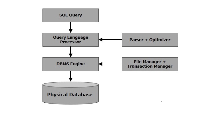
    SQL is not a database management system, but it is a query language which is used to store and retrieve the data from a database or in simple words SQL is a language that communicates with databases.

    SQL Examples

    Consider we have following CUSTOMERS table which stores customer”s ID, Name, Age, Salary, City and Country −

    ID Name Age Salary City Country
    1 Ramesh 32 2000.00 Maryland USA
    2 Mukesh 40 5000.00 New York USA
    3 Sumit 45 4500.00 Muscat Oman
    4 Kaushik 25 2500.00 Kolkata India
    5 Hardik 29 3500.00 Bhopal India
    6 Komal 38 3500.00 Saharanpur India
    7 Ayush 25 3500.00 Delhi India

    SQL makes it easy to manipulate this data using simple DML (Data Manipulation Language) Statements. For example, if we want to list down all the customers from USA then following will be the SQL query.

    SELECT * FROM CUSTOMERS WHERE country = ''USA
    

    This will produce the following result:

    ID Name Age Salary City Country
    1 Ramesh 32 2000.00 Maryland USA
    2 Mukesh 40 5000.00 New York USA

    SQL Online Editor

    We have provided SQL Online Editor which helps you to Edit and Execute the SQL code directly from your browser. Try to click the icon run button to run the following SQL code to be executed on CUSTOMERS table and print the records matching with the given condition.

    SELECT * FROM CUSTOMERS WHERE country = ''USA
    

    So now, you do not need to do a sophisticated setup to execute all the examples given in this tutorial because we are providing you Online SQL Editor, which allows you to edit your code and compile it online. You can try our .

    SQL Basic Commands

    We have a list of standard SQL commands to interact with relational databases, These commands are CREATE, SELECT, INSERT, UPDATE, DELETE, DROP and TRUNCATE and can be classified into the following groups based on their nature −

    Data Definition Language (DDL)

    A Data Definition Language (DDL) is a computer language which is used to create and modify the structure of database objects which include tables, views, schemas, and indexes etc.

    Command Description Demo
    CREATE Creates a new table, a view of a table, or other object in the database.
    ALTER Modifies an existing database object, such as a table.
    DROP Deletes an entire table, a view of a table or other objects in the database.
    TRUNCATE Truncates the entire table in a go. Demo

    Data Manipulation Language (DML)

    A Data Manipulation Language (DML) is a computer programming language which is used for adding, deleting, and modifying data in a database.

    Command Description Demo
    SELECT Retrieves certain records from one or more tables.
    INSERT Creates a record.
    UPDATE Modifies records.
    DELETE Deletes records.

    Data Control Language (DCL)

    Data Control Language (DCL) is a computer programming language which is used to control access to data stored in a database.

    Command Description Demo
    GRANT Gives a privilege to user Demo
    REVOKE Takes back privileges granted from user. Demo

    Why to Learn SQL?

    SQL (Structured Query Language) is a MUST for the students and working professionals to become a great Software Engineer specially when they are working in Software Development Domain. SQL is the most common language used almost in every application software including banking, finance, education, security etc. to store and manipulate data.

    SQL is fairly easy to learn, so if you are starting to learn any programming language then it is very much advised that you should also learn SQL and other Database related concepts to become a complete Software Programmer. There are many good reasons which makes SQL as the first choice of any programmer −

    SQL is the standard language for any Relational Database System. All the Relational Data Base Management Systems (RDBMS) like MySQL, MS Access, Oracle, Sybase, Informix, Postgres and SQL Server use SQL as their standard database language.

    Also, software industry is using different dialects of SQL, such as −

    • MS SQL Server using T-SQL,

    • Oracle using PL/SQL,

    • MS Access version of SQL is called JET SQL (native format) etc.

    SQL Applications

    SQL is one of the most widely used Query Language over the databases. SQL provides following functionality to the database programmers −

    • Execute different database queries against a database.

    • Define the data in a database and manipulate that data.

    • Create data in a relational database management system.

    • Access data from the relational database management system.

    • Create and drop databases and tables.

    • Create and maintain database users.

    • Create view, stored procedure, functions in a database.

    • Set permissions on tables, procedures and views.

    Who Should Learn SQL

    This SQL tutorial will help both students as well as working professionals who want to develop applications based on some databases like banking systems, support systems, information systems, web websites, mobile apps or personal blogs etc. We recommend reading this tutorial, in the sequence listed in the left side menu.

    Today, SQL is an essential language to learn for anyone involved in the software applicatipon development process including Software Developers, Software Designers, and Project Managers etc.

    Prerequisites to Learn SQL

    Though we have tried our best to present the SQL concepts in a simple and easy way, still before you start learning SQL concepts given in this tutorial, it is assumed that you are already aware about some basic concepts of computer science, what is a database, especially the basics of RDBMS and associated concepts.

    This tutorial will give you enough understanding on the various concepts of SQL along with suitable examples so that you can start your Software Development journey immediately after finishing this tutorial.

    SQL Online Quizzes

    This SQL tutorial helps you prepare for technical interviews and certification exams. We have provided various quizzes and assignments to check your learning level. Given quizzes have multiple choice type of questions and their answers with short explanation.

    Following is a sample quiz, try to attempt any of the given answers:

    Q 1 – The SQL programming language was developed by which of the following:

    Answer : C

    Explanation

    The SQL programming language was developed in the 1970s by IBM researchers Raymond Boyce and Donald Chamberlin.

    Start your online quiz .

    SQL Jobs and Opportunities

    SQL professionals are very much in high demand as the data turn out is increasing exponentially. Almost every major company is recruiting IT professionals having good experience with SQL.

    Average annual salary for a SQL professional is around $150,000. Though it can vary depending on the location. Following are the great companies who keep recruiting SQL professionals like Database Administrator (DBA), Database Developer, Database Testers, Data Scientist, ETL Developer, Database Migration Expert, Cloud Database Expert etc:

    • Google
    • Amazon
    • Netflix
    • Infosys
    • TCS
    • Tech Mahindra
    • Wipro
    • Pinterest
    • Uber
    • Trello
    • Many more…

    So, you could be the next potential employee for any of these major companies. We have developed a great learning material for SQL which will help you prepare for the technical interviews and certification exams based on SQL. So, start learning SQL using our simple and effective tutorial anywhere and anytime absolutely at your pace.

    Frequently Asked Questions about SQL

    There are some very Frequently Asked Questions(FAQ) about SQL, this section tries to answer them briefly.

    SQL skills help software programmers and data experts maintain, create and retrieve information from relational databases like MySQL, Oracle, MS SQL Server etc., which store data into columns and rows. It also allows them to access, update, manipulate, insert and modify data in efficient way.

    A relational database stores information in tabular form, with rows and columns representing different data attributes and the various relationships between the data values.

    There are 5 main types of commands. DDL (Data Definition Language) commands, DML (Data Manipulation Language) commands, and DCL (Data Control Language) commands, Transaction Control Language(TCL) commands and Data Query Language(DQL) commands.

    SQL is very easy to learn. You can learn SQL in as little as two to three weeks. However, it can take months of practice before you feel comfortable using it. Determining how long it takes to learn SQL also depends on how you plan to use it. Following this SQL tutorial will give you enough confidence to work on any software development related to database.

    SQL queries are also more flexible and powerful than Excel formulas and SQL is fast which can handle large amount of data. Unlike Excel, SQL can handle well over one million fields of data with ease.

    Here are the summarized list of tips which you can follow to start learning SQL.

    • First and the most important is to make your mind to learn SQL.
    • Install MySQL or MariaDB database on your computer system.
    • Follow our tutorial step by step starting from very begining.
    • Read more articles, watch online courses or buy a book on SQL to enhance your knowledge in SQL.
    • Try to develop a small software using PHP or Python which makes use of database.

    Following are four basic SQL Operations or SQL Statements.

    • SELECT statement selects data from database tables.
    • UPDATE statement updates existing data into database tables.
    • INSERT statement inserts new data into database tables.
    • DELETE statement deletes existing data from database tables.

    Following are following three SQL data types.

    • String Data types.
    • Numeric Data types.
    • Date and time Data types.

    You can use our simple and the best SQL tutorial to learn SQL. We have removed all the unnecessary complexity while teaching you SQL concepts. You can start learning it now .

    Khóa học lập trình tại Toidayhoc vừa học vừa làm dự án vừa nhận lương: Khóa học lập trình nhận lương tại trung tâm Toidayhoc

  • Khóa học miễn phí SQL – RDBMS Concepts nhận dự án làm có lương

    SQL – RDBMS Concepts

    Table of content


    What is RDBMS?

    RDBMS stands for Relational Database Management System. RDBMS is the basis for SQL, and for all modern database systems like MS SQL Server, IBM DB2, Oracle, MySQL, and Microsoft Access.

    A Relational database management system (RDBMS) is a database management system (DBMS) that is based on the relational model as introduced by E. F. Codd in 1970.

    What is a Table?

    The data in an RDBMS is stored in database objects known as tables. This table is basically a collection of related data entries and it consists of numerous columns and rows.

    Remember, a table is the most common and simplest form of data storage in a relational database. Following is an example of a CUSTOMERS table which stores customer”s ID, Name, Age, Salary, City and Country −

    ID Name Age Salary City Country
    1 Ramesh 32 2000.00 Hyderabad India
    2 Mukesh 40 5000.00 New York USA
    3 Sumit 45 4500.00 Muscat Oman
    4 Kaushik 25 2500.00 Kolkata India
    5 Hardik 29 3500.00 Bhopal India
    6 Komal 38 3500.00 Saharanpur India
    7 Ayush 25 3500.00 Delhi India
    8 Javed 29 3700.00 Delhi India

    What is a Field?

    Every table is broken up into smaller entities called fields. A field is a column in a table that is designed to maintain specific information about every record in the table.

    For example, our CUSTOMERS table consists of different fields like ID, Name, Age, Salary, City and Country.

    What is a Record or a Row?

    A record is also called as a row of data is each individual entry that exists in a table. For example, there are 7 records in the above CUSTOMERS table. Following is a single row of data or record in the CUSTOMERS table −

    ID Name Age Salary City Country
    1 Ramesh 32 2000.00 Hyderabad India

    A record is a horizontal entity in a table.

    What is a Column?

    A column is a vertical entity in a table that contains all information associated with a specific field in a table.

    For example, our CUSTOMERS table have different columns to represent ID, Name, Age, Salary, City and Country.

    What is a NULL Value?

    A NULL value in a table is a value in a field that appears to be blank, which means a field with a NULL value is a field with no value.

    It is very important to understand that a NULL value is different than a zero value or a field that contains spaces. A field with a NULL value is the one that has been left blank during a record creation. Following table has three records where first record has NULL value for the salary and second record has a zero value for the salary.

    ID Name Age Salary City Country
    1 Ramesh 32 Hyderabad India
    2 Mukesh 40 00.00 New York USA
    3 Sumit 45 4500.00 Muscat Oman

    SQL Constraints

    Constraints are the rules enforced on data columns on a table. These are used to limit the type of data that can go into a table. This ensures the accuracy and reliability of the data in the database.

    Constraints can either be column level or table level. Column level constraints are applied only to one column whereas, table level constraints are applied to the entire table.

    Following are some of the most commonly used constraints available in SQL −

    S.No. Constraints
    1

    Ensures that a column cannot have a NULL value.

    2

    Provides a default value for a column when none is specified.

    3

    Ensures that all the values in a column are different.

    4

    Uniquely identifies each row/record in a database table.

    5

    Uniquely identifies a row/record in any another database table.

    6

    Ensures that all values in a column satisfy certain conditions.

    7

    Used to create and retrieve data from the database very quickly.

    Data Integrity

    The following categories of data integrity exist with each RDBMS −

    • Entity Integrity − This ensures that there are no duplicate rows in a table.

    • Domain Integrity − Enforces valid entries for a given column by restricting the type, the format, or the range of values.

    • Referential integrity − Rows cannot be deleted, which are used by other records.

    • User-Defined Integrity − Enforces some specific business rules that do not fall into entity, domain or referential integrity.

    Database Normalization

    Database normalization is the process of efficiently organizing data in a database. There are two reasons of this normalization process −

    • Eliminating redundant data, for example, storing the same data in more than one table.

    • Ensuring data dependencies make sense.

    Both these reasons are worthy goals as they reduce the amount of space a database consumes and ensures that data is logically stored. Normalization consists of a series of guidelines that help guide you in creating a good database structure.

    Normalization guidelines are divided into normal forms; think of a form as the format or the way a database structure is laid out. The aim of normal forms is to organize the database structure, so that it complies with the rules of first normal form, then second normal form and finally the third normal form.

    It is your choice to take it further and go to the Fourth Normal Form, Fifth Normal Form and so on, but in general, the Third Normal Form is more than enough for a normal Database Application.


    Khóa học lập trình tại Toidayhoc vừa học vừa làm dự án vừa nhận lương: Khóa học lập trình nhận lương tại trung tâm Toidayhoc

  • Khóa học miễn phí SQL – Overview nhận dự án làm có lương

    SQL – Overview

    Table of content


    What is SQL?

    SQL (Structured Query Language) is a language to operate databases; it includes Database Creation, Database Deletion, Fetching Data Rows, Modifying & Deleting Data rows, etc.

    SQL stands for Structured Query Language which is a computer language for storing, manipulating and retrieving data stored in a relational database. SQL was developed in the 1970s by IBM Computer Scientists and became a standard of the American National Standards Institute (ANSI) in 1986, and the International Organization for Standardization (ISO) in 1987.

    Though SQL is an ANSI (American National Standards Institute) standard language, but there are many different dialects of the SQL language like MS SQL Server is using T-SQL and Oracle is using PL/SQL.

    SQL is the standard language to communicate with Relational Database Systems. All the Relational Database Management Systems (RDMS) like MySQL, MS Access, Oracle, Sybase, Informix, Postgres and SQL Server use SQL as their Standard Database Language.

    Why SQL?

    SQL is widely popular because it offers the following advantages −

    • Allows users to access data in the relational database management systems.

    • Allows users to describe the data.

    • Allows users to define the data in a database and manipulate that data.

    • Allows to embed within other languages using SQL modules, libraries & pre-compilers.

    • Allows users to create and drop databases and tables.

    • Allows users to create view, stored procedure, functions in a database.

    • Allows users to set permissions on tables, procedures and views.

    A Brief History of SQL

    • 1970 − Dr. Edgar F. “Ted” Codd of IBM is known as the father of relational databases. He described a relational model for databases.

    • 1974 − Structured Query Language (SQL) appeared.

    • 1978 − IBM worked to develop Codd”s ideas and released a product named System/R.

    • 1986 − IBM developed the first prototype of relational database and standardized by ANSI. The first relational database was released by Relational Software which later came to be known as Oracle.

    • 1987 − SQL became the part of the International Organization for Standardization (ISO).

    How SQL Works?

    When you are executing an SQL command for any RDBMS, the system determines the best way to carry out your request and SQL engine figures out how to interpret the task.

    There are various components included in this process. These components are −

    • Query Dispatcher
    • Optimization Engines
    • Classic Query Engine
    • SQL Query Engine, etc.

    A classic query engine handles all the non-SQL queries, but a SQL query engine won”t handle logical files. Following is a simple diagram showing the SQL Architecture −

    SQL Architecture

    Khóa học lập trình tại Toidayhoc vừa học vừa làm dự án vừa nhận lương: Khóa học lập trình nhận lương tại trung tâm Toidayhoc

  • Khóa học miễn phí SQL – Databases nhận dự án làm có lương

    SQL Databases

    Table of content


    SQL Databases

    SQL or Relational databases are used to store and manage the data objects that are related to one another, i.e. the process of handling data in a relational database is done based on a relational model.

    This relational model is an approach to manage data in a structured way (using tables). A system used to manage these is known as Relational Database Management System (RDBMS).

    SQL Database Table Structure

    SQL database server stores data in table form. are database objects used to collect data in Row and Column format. Rows represent the entities whereas columns define the attributes of each entity in a table.

    Columns: Columns are vertical elements in a table. Each column in a table holds specific attribute information, and column properties such as column name and data types (Integer, Char, String, etc).

    Rows: Rows are horizontal elements in a table and users can add data or retrieve by executing SQL queries.

    Types of SQL Databases

    There are many popular RDBMS available to work with. Some of the most popular RDBMS are listed below −

    • MySQL
    • MS SQL Server
    • ORACLE
    • MS ACCESS
    • PostgreSQL
    • SQLite

    This SQL databases tutorial gives a brief overview of these RDBMS specified above. This would help you to compare their basic features.

    MySQL

    is an open source SQL database, which is developed by a Swedish company, MySQL AB. MySQL is pronounced as “my ess-que-ell,” in contrast with SQL, pronounced “sequel.”

    MySQL is supporting many different platforms including Microsoft Windows, the major Linux distributions, UNIX, and Mac OS X.

    MySQL has free and paid versions, depending on its usage (non-commercial/commercial) and features. MySQL comes with a very fast, multi-threaded, multi-user and robust SQL database server.

    History

    • 1994 – Development of MySQL by Michael Widenius & David Axmark beginning in 1994.

    • 1995 – First internal release on 23rd May 1995.

    • 1998 – Windows Version was released on the 8th January 1998 for Windows 95 and NT.

    • 2001 – Version 3.23 released beta from June 2000, and production release January 2001.

    • 2003 – Version 4.0 was released on August 2002 as beta, and as production release on March 2003 (unions).

    • 2004 – Version 4.1 was released on June 2004 as beta, and as production release on October 2004.

    • 2005 – Version 5.0 was released on March 2005 as beta, and as a production release on October 2005.

    • 2008 – Sun Microsystems acquired MySQL AB on the 26th February 2008, and Oracle Version 5.1 had its production release on 27th November 2008.

    • 2010 – Oracle acquired Sun Microsystems on 27th January 2010 and general availability of version 5.5 was on 3rd December 2010.

    • 2013 – General availability of Version 5.6 was enabled on 5th February 2013

    • 2015 – General availability of Version 5.7 was enabled on 21st October 2015

    • 2018 – General availability of Version 8.0 was enabled on 19th April 2018, and is the latest version of MySQL.

    Features

    • High Performance.
    • High Availability.
    • Scalability and Flexibility Run anything.
    • Robust Transactional Support.
    • Web and Data Warehouse Strengths.
    • Strong Data Protection.
    • Comprehensive Application Development.
    • Management Ease.
    • Open Source Freedom and 24 x 7 Support.
    • Lowest Total Cost of Ownership.

    MS SQL Server

    is a Relational Database Management System developed by Microsoft Inc. Its primary query languages are −

    • T-SQL
    • ANSI SQL

    History

    • 1987 – Sybase releases SQL Server for UNIX.

    • 1988 – Microsoft, Sybase, and Aston-Tate port SQL Server to OS/2.

    • 1989 – Microsoft, Sybase, and Aston-Tate release SQL Server 1.0 for OS/2.

    • 1990 – SQL Server 1.1 is released with support for Windows 3.0 clients.

    • 2000 – Microsoft releases SQL Server 2000.

    • 2001 – Microsoft releases XML for SQL Server Web Release 1 (download).

    • 2002 – Microsoft releases SQLXML 2.0 (renamed from XML for SQL Server).

    • 2002 – Microsoft releases SQLXML 3.0.

    • 2006 – Microsoft releases SQL Server 2005 on January 14, 2006.

    • 2008 – Microsoft releases SQL Server 2008 on November 6, 2008. And R2 version is released on July 20, 2010.

    • 2012 – Microsoft releases SQL Server 2012 on May 20, 2012.

    • 2014 – Microsoft releases SQL Server 2014 on June 5, 2014.

    • 2016 – Microsoft releases SQL Server 2016 on June 1, 2016.

    • 2017 – Microsoft releases SQL Server 2017 on September 29, 2017.

    • 2019 – Microsoft releases SQL Server 2019 on November 4, 2019.

    • 2022 – Microsoft releases SQL Server 2022 on November 16, 2022.

    Features

    • High Performance
    • High Availability
    • Database mirroring
    • Database snapshots
    • CLR integration
    • Service Broker
    • DDL triggers
    • Ranking functions
    • Row version-based isolation levels
    • XML integration
    • TRY…CATCH
    • Database Mail

    ORACLE

    is a very large multi-user based database management system. Oracle is a relational database management system developed by ”Oracle Corporation”.

    Oracle works to efficiently manage its resources, a database of information among the multiple clients requesting and sending data in the network.

    It is an excellent database server choice for client/server computing. Oracle supports all major operating systems for both clients and servers, including MSDOS, NetWare, UnixWare, OS/2 and most UNIX flavors.

    History

    Oracle began in 1977 and celebrating its 46 wonderful years in the industry (from 1977 to 2023).

    • 1977 – Larry Ellison, Bob Miner and Ed Oates founded Software Development Laboratories to undertake development work.

    • 1979 – Version 2.0 of Oracle was released and it became first commercial relational database and first SQL database. The company changed its name to Relational Software Inc. (RSI).

    • 1981 – RSI started developing tools for Oracle.

    • 1982 – RSI was renamed to Oracle Corporation.

    • 1983 – Oracle released version 3.0, rewritten in C language and ran on multiple platforms.

    • 1984 – Oracle version 4.0 was released. It contained features like concurrency control – multi-version read consistency, etc.

    • 1985 – Oracle version 4.0 was released. It contained features like concurrency control – multi-version read consistency, etc.

    • 2007 – Oracle released Oracle11g. The new version focused on better partitioning, easy migration, etc.

    • 2013 – Oracle Database 12c R1 version was released in July, 2013; and R2 version was released on cloud in August 2016, and released on-prem in March 2017.

    • 2018 – Oracle Database 18c version was initially released in July 2018.

    • 2019 – Oracle Database 19c version was released in February 2019.

    • 2020 – Oracle Database 21c version was released in December 2020.

    • 2023 – Oracle Database 23c version was released in April 2023.

    Features

    • Concurrency
    • Read Consistency
    • Locking Mechanisms
    • Quiesce Database
    • Portability
    • Self-managing database
    • SQL*Plus
    • ASM
    • Scheduler
    • Resource Manager
    • Data Warehousing
    • Materialized views
    • Bitmap indexes
    • Table compression
    • Parallel Execution
    • Analytic SQL
    • Data mining
    • Partitioning

    MS ACCESS

    Microsoft Access is one of the most popular Microsoft products. It is an entry-level database management software. It is not only inexpensive but also a powerful database for small-scale projects.

    uses the Jet database engine, which utilizes a specific SQL language dialect (sometimes referred to as Jet SQL). It comes with the professional edition of MS Office package. MS Access has easy to-use intuitive graphical interface.

    • 1992 – Access version 1.0 was released.

    • 1993 – Access 1.1 released to improve compatibility with inclusion the Access Basic programming language.

    • The most significant transition was from Access 97 to Access 2000.

    • 2007 – Access 2007, a new database format was introduced ACCDB which supports complex data types such as multi valued and attachment fields.

    • 2010 – Microsoft Access 2010 introduced a new version of the ACCDB format supported hosting Access Web services on a SharePoint 2010 server.

    • 2013 – Microsoft Access 2013 offers traditional Access desktop applications plus a significantly updated SharePoint 2013 web service

    • 2021 – Microsoft Access is no longer included in one-time purchase version of Microsoft Office 2021, but remains within the Microsoft 365 counterpart.

    Features

    • Users can create tables, queries, forms and reports and connect them together with macros.

    • Option of importing and exporting the data to many formats including Excel, Outlook, ASCII, dBase, Paradox, FoxPro, SQL Server, Oracle, ODBC, etc.

    • There is also the Jet Database format (MDB or ACCDB in Access 2007), which can contain the application and data in one file. This makes it very convenient to distribute the entire application to another user, who can run it in disconnected environments.

    • Microsoft Access offers parameterized queries. These queries and Access tables can be referenced from other programs like VB6 and .NET through DAO or ADO.

    • The desktop editions of Microsoft SQL Server can be used with Access as an alternative to the Jet Database Engine.

    • Microsoft Access is a file server-based database. Unlike the client-server relational database management systems (RDBMS), Microsoft Access does not implement database triggers, stored procedures or transaction logging.

    PostgreSQL

    PostgreSQL is object relational database management system (ORDBMS) that supports both relational (SQL) and non-relational (JSON) query. It is a highly stable database that is developed based on the POSTGRES, version 4.2 released by the Computer Science Department in University of Berkeley, California. This database is a popular database or data warehouse for many applications.

    History

    • 1970s – Ingres was being developed in Computer Science department of University of Berkeley as a research project which ended in 1985.

    • 1985 – A post-Ingres project, namely POSTGRES, has been initiated to address the issues in the older database systems. This project aimed to fully support datatypes and define them to establish relationships between the objects of the database. POSTGRES also was able to retrieve data using rules.

    • 1989 – POSTGRES Version 1 was released to the small number of users.

    • 1990 – POSTGRES Version 2 was released again with rewritten rules.

    • 1994 – With the increase in users, POSTGRES Version 4.2 was released, ending the project with it.

    • 1994 – Andrew Yu and Jolly Chen, students of University of Berkeley, replaced the POSTQUEL query language that run POSTGRES, with the SQL language, creating Postgres95.

    • 1995 – Postgres95”s first version was released with a more liberal license.

    • 1996 – The project was renamed to PostgreSQL to support SQL.

    • 1997 – The first version of PostgreSQL version 6.0 was released.

    • Since then, next versions of the project is released as free and open-source software PostgreSQL License.

    • 2000 – PostgreSQL version 7.0 was released on July 8th, 2000. This version had the most changes in features until then. Major changes made were foreign keys were implemented, optimizer had been improved, psql had been updated, and JOIN syntax is now supported.

    • 2005 – The version 8.0 was released on January 19th, 2005. Changes in this version include, the server can now be run on Microsoft natively, savepoints are introduced, Point-in-time recovery, tablespaces, improved buffer managements, checkpoints, changing column types is introduced, etc.

    • 2010 – PostgreSQL version 9.0 was released on 20th September, 2010.

    • 2017 – Version 10.0 was released on 5th October, 2017. Major improvements include: logical replication, declarative table partitioning, improved query parallelism, significant improvements in general performance, etc.

    • 2018 – PostgreSQL version 11.0 was released on 18th October, 2018.

    • 2019 – PostgreSQL version 12.0 was released on 3rd October, 2019.

    • 2020 – PostgreSQL version 13.0 was released on 24th September, 2020.

    • 2021 – PostgreSQL version 14.0 was released on 30th September, 2021.

    • 2022 – PostgreSQL version 15.0 was released on 13th October, 2022.

    Features

    • PostgreSQL supports advanced data types.
    • It possesses high levels of resilience, integrity and correctness of the data.
    • It contains Multi-Version Concurrency Control (MVCC)
    • Point in time recovery
    • Granular Access Controls
    • Asynchronous Replication
    • Nested transactions
    • Online backups
    • Refined query optimizer
    • Write ahead logging
    • It supports international character sets, multi-byte character encodings, Unicode.
    • It is locale-aware for sorting, case-sensitivity, and formatting.
    • Highly scalable.

    SQLite

    SQLite is an embedded relational database system. It is referred to as a lightweight database as it is not more than 500kB in size, which is way less than other relational databases. This database is an in-memory open source library; which is why it can access the files stored in it directly and the source code for it is available in the public domain.

    History

    • 2000 – SQLite 1.0 was released with GNU Database Manager. Dr. Richard Hipp designed it in the same year to create a database that requires no administration.

    • 2001 – SQLite 2.0 was released which contained a custom B-Tree implementation instead of GNU Database Manager, adding transaction capability to the database.

    • 2003 – SQLite 3.0 was released with major improvements like internalization, manifest typing etc.

    • 2011 – Hipp announced his plans to introduce a non-relational interface to SQLite.

    • 2018 – SQLite adopted the Code of Conduct from the Rule of Saint Benedict which was later renamed as Code of Ethics due to some controversies.

    • Despite such controversies, newer versions of SQLite 3.x are being released continuously with better features and improvements.

    • 2023 – The latest version of SQLite is 3.42.0 which was released on 16th July, 2023..

    Features

    • SQLite is an open source library witten in ANSI C.
    • It works on cross-platforms, making it easier to port to other systems.
    • The source code for SQLite is available in public domain.
    • Transactions in SQLite are atomic, consistent, isolated and durable even when the system crashes for any reason.
    • This database does not need any configuration or administration.
    • SQLite is server less, unlike other relational databases. It is linked with application that accesses it. The application directly interacts with the SQLite to read and write on files stored in the disk.
    • It has a simple and easy to use API.
    • In some cases, SQLite is faster than direct filesystem I/O operations.
    • SQLite is self contained, i.e. it is not dependent on any external libraries or operating systems.
    • Uses a stand-alone command line interface (CLI) client to administer SQLite.

    Benefits of Using SQL Database

    Relational databases are the most popular and preferred databases used for data storage. There are many benefits to using SQL database, including:

    Enhanced Flexibility

    Relational databases utilize Data Definition Language (DDL) to modify data stored in tables in real time. The most important thing users can easily add new tables and columns, rename, and implement various changes without disrupting ongoing database operations.

    Data Consistency

    Data Consistency is another important benefit of using SQL databases because it maintains data consistency across applications and server instances.

    Minimum Data Redundancy

    Relational Database Management Systems (RDBMS) use the normalization process to reduce data redundancy. This approach eliminates anomalies in Data stores in the Database.

    Optimized Performance

    Relational databases offer a range of value-added features that boast minimal memory usage, reduced storage costs, and high processor speed.

    Higher Compatibility

    Relational databases offer higher compatibility for integration with modern technologies.

    Scalability

    Higher scalability is another feature that makes Relational databases most preferred.


    Khóa học lập trình tại Toidayhoc vừa học vừa làm dự án vừa nhận lương: Khóa học lập trình nhận lương tại trung tâm Toidayhoc

  • Khóa học miễn phí SQL – Create Database nhận dự án làm có lương

    SQL – CREATE Database

    Table of content


    A database is a structured collection of data that is stored in a computer system. They are used to store and retrieve the data efficiently. Databases can be created using different query languages, and is one such language.

    CREATE Database Statement

    The CREATE DATABASE statement is a DDL (Data Definition Language) statement used to create a new database in SQL. If you are creating your database on Linux or Unix, then database names are case-sensitive, even though SQL keywords are case-insensitive. If you are working on Windows then this restriction does not apply.

    Syntax

    Following is the syntax to create a database in SQL

    CREATE DATABASE DatabaseName;
    

    Here, the DatabaseName is the name of the database that we want to create. The database name can contain any valid identifiers, such as number, letters, or underscores. But a DatabaseName cannot be a keyword available in SQL.

    While creating a database, you may encounter an error such as ERROR 1044 (42000): Access denied for user ”krishna”@”localhost” to database ”DatabaseName”, this means that you do not have the necessary privileges to create a database. To create a database, you need to have admin previleges.

    Example

    Following is an example to create a database testDB using SQL CREATE DATABASE statement −

    CREATE DATABASE testDB;
    

    List Databases using SQL

    Once the database testDB is created, you can check it in the list of databases using SQL command SHOW DATABASES;.

    Syntax

    SHOW DATABASES;
    

    Output

    The output will be displayed as −

    Database
    master
    performance_schema
    information_schema
    mysql
    testDB

    Use/Select Databases using SQL

    We can now set the testDB as the default database by using the USE statement in SQL.

    Syntax

    USE testDB;
    

    That”s it! we have successfully created a database in SQL. Now, we can create tables and other database objects within this new database.


    Khóa học lập trình tại Toidayhoc vừa học vừa làm dự án vừa nhận lương: Khóa học lập trình nhận lương tại trung tâm Toidayhoc

  • Khóa học miễn phí SQL – Syntax nhận dự án làm có lương

    SQL – Syntax

    Table of content


    What is SQL Syntax?

    SQL syntax is a unique set of rules and guidelines to be followed while writing SQL statements. This tutorial gives you a quick start with SQL by listing all the basic SQL Syntax.

    All the SQL statements start with any of the keywords like SELECT, INSERT, UPDATE, DELETE, ALTER, DROP, CREATE, USE, SHOW and all the statements end with a semicolon (;).

    Case Sensitivity

    The most important point to be noted here is that SQL is case insensitive, which means SELECT and Select have same meaning in SQL statements. Whereas, MySQL makes difference in table names. So, if you are working with MySQL, then you need to give table names as they exist in the database.

    SQL Table

    Let us consider a table with the name CUSTOMERS shown below, and use it as a reference to demonstrate all the SQL Statements on the same.

    ID NAME AGE ADDRESS SALARY
    1 Ramesh 32 Ahmedabad 2000.00
    2 Khilan 25 Delhi 1500.00
    3 kaushik 23 Kota 2000.00
    4 Chaitali 25 Mumbai 6500.00
    5 Hardik 27 Bhopal 8500.00
    6 Komal 22 Hyderabad 4500.00
    7 Muffy 24 Indore 10000.00

    SQL Statements

    This tutorial lists down various SQL statements. Most of them are compatible with MySQL, Oracle, Postgres and SQL Server databases.

    All the SQL statements require a semicolon (;) at the end of each statement. Semicolon is the standard way to separate different SQL statements which allows to include multiple SQL statements in a single line.

    All the SQL Statements given in this tutorial have been tested with a MySQL server on Linux and Windows.

    SQL CREATE DATABASE Statement

    To store data within a database, you first need to create it. This is necessary to individualize the data belonging to an organization.

    You can create a database using the following syntax −

    CREATE DATABASE database_name;
    

    Let us try to create a sample database sampleDB in SQL using the CREATE DATABASE statement −

    CREATE DATABASE sampleDB
    

    SQL USE Statement

    Once the database is created, it needs to be used in order to start storing the data accordingly. Following is the syntax to change the current location to required database −

    USE database_name;
    

    We can set the previously created sampleDB as the default database by using the USE statement in SQL −

    USE sampleDB;
    

    SQL DROP DATABASE Statement

    If a database is no longer necessary, you can also delete it. To delete/drop a database, use the following syntax −

    DROP DATABASE database_name;
    

    You can also drop the sampleDB database by using the DROP DATABASE statement in SQL −

    DROP DATABASE sampleDB;
    

    SQL CREATE TABLE Statement

    In an SQL driven database, the data is stored in a structured manner, i.e. in the form of tables. To create a table, following syntax is used −

    CREATE TABLE table_name(
       column1 datatype,
       column2 datatype,
       column3 datatype,
       .....
       columnN datatype,
       PRIMARY KEY( one or more columns )
    );
    

    The following code block is an example, which creates a CUSTOMERS table given above, with an ID as a primary key and NOT NULL are the constraints showing that these fields cannot be NULL while creating records in this table −

    CREATE TABLE CUSTOMERS(
       ID   INT              NOT NULL,
       NAME VARCHAR (20)     NOT NULL,
       AGE  INT              NOT NULL,
       ADDRESS  CHAR (25) ,
       SALARY   DECIMAL (18, 2),
       PRIMARY KEY (ID)
    );
    

    SQL DESC Statement

    Every table in a database has a structure of its own. To display the structure of database tables, we use the DESC statements. Following is the syntax −

    DESC table_name;
    

    The DESC Statement, however, only works in few RDBMS systems; hence, let us see an example by using DESC statement in the MySQL server −

    DESC CUSTOMERS;
    

    SQL INSERT INTO Statement

    The SQL INSERT INTO Statement is used to insert data into database tables. Following is the syntax −

    INSERT INTO table_name( column1, column2....columnN)
    VALUES ( value1, value2....valueN);
    

    The following example statements would create seven records in the empty CUSTOMERS table.

    INSERT INTO CUSTOMERS VALUES
    (1, ''Ramesh'', 32, ''Ahmedabad'', 2000.00 ),
    (2, ''Khilan'', 25, ''Delhi'', 1500),
    (3, ''kaushik'', 23, ''Kota'', 2000),
    (4, ''Chaitali'', 25, ''Mumbai'', 6500),
    (5, ''Hardik'', 27, ''Bhopal'', 8500),
    (6, ''Komal'', 22, ''Hyderabad'', 4500),
    (7, ''Muffy'', 24, ''Indore'', 10000);
    

    SQL SELECT Statement

    In order to retrieve the result-sets of the stored data from a database table, we use the SELECT statement. Following is the syntax −

    SELECT column1, column2....columnN FROM table_name;
    

    To retrieve the data from CUSTOMERS table, we use the SELECT statement as shown below.

    SELECT * FROM CUSTOMERS;
    

    SQL UPDATE Statement

    When the stored data in a database table is outdated and needs to be updated without having to delete the table, we use the UPDATE statement. Following is the syntax −

    UPDATE table_name
    SET column1 = value1, column2 = value2....columnN=valueN
    [ WHERE  CONDITION ];
    

    To see an example, the following query will update the ADDRESS for a customer whose ID number is 6 in the table.

    UPDATE CUSTOMERS SET ADDRESS = ''Pune'' WHERE ID = 6;
    

    SQL DELETE Statement

    Without deleting the entire table from the database, you can also delete a certain part of the data by applying conditions. This is done using the DELETE FROM statement. Following is the syntax −

    DELETE FROM table_name WHERE  {CONDITION};
    

    The following code has a query, which will DELETE a customer, whose ID is 6.

    DELETE FROM CUSTOMERS WHERE ID = 6;
    

    SQL DROP TABLE Statement

    To delete a table entirely from a database when it is no longer needed, following syntax is used −

    DROP TABLE table_name;
    

    This query will drop the CUSTOMERS table from the database.

    DROP TABLE CUSTOMERS;
    

    SQL TRUNCATE TABLE Statement

    The TRUNCATE TABLE statement is implemented in SQL to delete the data of the table but not the table itself. When this SQL statement is used, the table stays in the database like an empty table. Following is the syntax −

    TRUNCATE TABLE table_name;
    

    Following query delete all the records of the CUSTOMERS table −

    TRUNCATE TABLE CUSTOMERS;
    

    SQL ALTER TABLE Statement

    The ALTER TABLE statement is used to alter the structure of a table. For instance, you can add, drop, and modify the data of a column using this statement. Following is the syntax −

    ALTER TABLE table_name
    {ADD|DROP|MODIFY} column_name {data_type};
    

    Following is the example to ADD a New Column to the CUSTOMERS table using ALTER TABLE command −

    ALTER TABLE CUSTOMERS ADD SEX char(1);
    

    SQL ALTER TABLE Statement (Rename)

    The ALTER TABLE statement is also used to change the name of a table as well. Use the syntax below −

    ALTER TABLE table_name RENAME TO new_table_name;
    

    Following is the example to RENAME the CUSTOMERS table using ALTER TABLE command −

    ALTER TABLE CUSTOMERS RENAME TO NEW_CUSTOMERS;
    

    SQL DISTINCT Clause

    The DISTINCT clause in a database is used to identify the non-duplicate data from a column. Using the SELECT DISTINCT statement, you can retrieve distinct values from a column. Following is the syntax −

    SELECT DISTINCT column1, column2....columnN FROM   table_name;
    

    As an example, let us use the DISTINCT keyword with a SELECT query. The repetitive salary 2000.00 will only be retrieved once and the other record is ignored.

    SELECT DISTINCT SALARY FROM CUSTOMERS ORDER BY SALARY;
    

    SQL WHERE Clause

    The WHERE clause is used to filter rows from a table by applying a condition. Following is the syntax to retrieve filtered rows from a table −

    SELECT column1, column2....columnN
    FROM   table_name
    WHERE  CONDITION;
    

    The following query is an example to fetch all the records from CUSTOMERS table where the salary is greater than 2000, using the SELECT statement −

    SELECT ID, NAME, SALARY
    FROM CUSTOMERS
    WHERE SALARY > 2000;
    

    SQL AND/OR Operators

    The AND/OR Operators are used to apply multiple conditions in the WHERE clause. Following is the syntax −

    SELECT column1, column2....columnN
    FROM   table_name
    WHERE  CONDITION-1 {AND|OR} CONDITION-2;
    

    The following query is an example to fetch all the records from CUSTOMERS table where the salary is greater than 2000 AND age is less than 25, using the SELECT statement −

    SELECT ID, NAME, SALARY FROM CUSTOMERS WHERE SALARY > 2000 AND age < 25;
    

    SQL IN Clause

    The IN Operator is used to check whether the data is present in the column or not, using the WHERE clause. Following is the syntax −

    SELECT column1, column2....columnN
    FROM   table_name
    WHERE  column_name IN (val-1, val-2,...val-N);
    

    For an example, we want to display records with NAME equal to ”Khilan”, ”Hardik” and ”Muffy” (string values) using IN operator as follows −

    SELECT * FROM CUSTOMERS
    WHERE NAME IN (''Khilan'', ''Hardik'', ''Muffy'');
    

    SQL BETWEEN Clause

    The BETWEEN Operator is used to retrieve the values from a table that fall in a certain range, using the WHERE clause. Following is the syntax −

    SELECT column1, column2....columnN
    FROM   table_name
    WHERE  column_name BETWEEN val-1 AND val-2;
    

    Let us try to the BETWEEN operator to retrieve CUSTOMERS records whose AGE is between 20 and 25.

    SELECT * FROM CUSTOMERS WHERE AGE BETWEEN 20 AND 25;
    

    SQL LIKE Clause

    The LIKE Operator is used to retrieve the values from a table that match a certain pattern, using the WHERE clause. Following is the syntax −

    SELECT column1, column2....columnN
    FROM   table_name
    WHERE  column_name LIKE { PATTERN };
    

    As an example, let us try to display all the records from the CUSTOMERS table, where the SALARY starts with 200.

    SELECT * FROM CUSTOMERS WHERE SALARY LIKE ''200%
    

    SQL ORDER BY Clause

    The ORDER BY Clause is used to arrange the column values in a given/specified order. Following is the syntax −

    SELECT column1, column2....columnN
    FROM   table_name
    WHERE  CONDITION
    ORDER BY column_name {ASC|DESC};
    

    In the following example we are trying to sort the result in an ascending order by the alphabetical order of customer names −

    SELECT * FROM CUSTOMERS ORDER BY NAME ASC;
    

    SQL GROUP BY Clause

    The GROUP BY Clause is used to group the values of a column together. Following is the syntax −

    SELECT SUM(column_name)
    FROM   table_name
    WHERE  CONDITION
    GROUP BY column_name;
    

    We are trying to group the customers by their age and calculate the average salary for each age group using the following query −

    SELECT ADDRESS, AGE, SUM(SALARY)
    AS TOTAL_SALARY FROM CUSTOMERS
    GROUP BY ADDRESS, AGE;
    

    SQL COUNT Function

    The COUNT Function gives the number of non-null values present in the specified column. Following is the syntax −

    SELECT COUNT(column_name)
    FROM   table_name
    WHERE  CONDITION;
    

    Let us see an example −

    SELECT AGE, COUNT(Name) FROM CUSTOMERS GROUP BY AGE;
    

    SQL HAVING Clause

    The HAVING clause is also used to filter a group of rows by applying a condition. Following is the syntax −

    SELECT SUM(column_name)
    FROM   table_name
    WHERE  CONDITION
    GROUP BY column_name
    HAVING (arithematic function condition);
    

    In the following example, we are trying to retrieve all records from the CUSTOMERS table where the sum of their salary is greater than 5000 −

    SELECT ADDRESS, AGE, SUM(SALARY) AS
    TOTAL_SALARY FROM CUSTOMERS GROUP BY
    ADDRESS, AGE HAVING TOTAL_SALARY >=5000
    ORDER BY TOTAL_SALARY DESC;
    

    SQL CREATE INDEX Statement

    To create an index on a database table, SQL provides the CREATE INDEX statement. Following is the syntax −

    CREATE UNIQUE INDEX index_name
    ON table_name ( column1, column2,...columnN);
    

    Let us create an index for the column named ”NAME” in the existing CUSTOMERS table using the following query −

    CREATE INDEX sample_index on CUSTOMERS(NAME);
    

    SQL DROP INDEX Statement

    The DROP INDEX statement is used to drop an index from a table. Following is the syntax −

    DROP INDEX index_name ON table_name;
    

    Let us drop the index we created previously for the column named ”NAME” in the existing CUSTOMERS table using the following query −

    DROP INDEX sample_index on CUSTOMERS;
    

    Khóa học lập trình tại Toidayhoc vừa học vừa làm dự án vừa nhận lương: Khóa học lập trình nhận lương tại trung tâm Toidayhoc

  • Khóa học miễn phí SQL – Operators nhận dự án làm có lương

    SQL – Operators

    Table of content


    What is SQL Operator?

    An SQL operator is a reserved word or a character used primarily in an SQL statement”s WHERE clause to perform operation(s), such as comparisons and arithmetic operations. These Operators are used to specify conditions in an SQL statement and to serve as conjunctions for multiple conditions in a statement.

    An SQL operator can be either a unary or binary operator. A unary operator (example unary + or unary – ) uses only one operand to perform the unary operation, whereas the binary operator (example + or – etc) uses two operands to perform the binary operation.

    Types of Operator in SQL

    supports following types of operators:

    • Operators used to negate conditions

    SQL Arithmetic Operators

    SQL Arithmetic Operators are used to perform mathematical operations on the numerical values. SQL provides following operators to perform mathematical operations.

    Here is a list of all the arithmetic operators available in SQL.

    Operator Description Example
    + Addition 10 + 20 = 30
    Subtraction 20 – 30 = -10
    * Multiplication 10 * 20 = 200
    / Division 20 / 10 = 2
    % Modulus 5 % 2 = 1

    SQL Comparison Operators

    SQL Comparison Operators test whether two given expressions are the same or not. These operators are used in SQL conditional statements while comparing one expression with another and they return a Boolean value which can be either TRUE or FALSE. The result of an SQL comparison operation can be UNKNOWN when one or another operand has it”s value as NULL.

    Here is a list of all the comparison operators available in SQL.

    Operator Description Example
    = Equal to 5 = 5 returns TRUE
    != Not equal 5 != 6 returns TRUE
    <> Not equal 5 <> 4 returns TRUE
    > Greater than 4 > 5 returns FALSE
    < Less than 4 < 5 returns TRUE
    >= Greater than or equal to 4 >= 5 returns FALSE
    <= Less than or equal to 4 <= 5 returns TRUE
    !< Not less than 4 !< 5 returns FALSE
    !> Not greater than 4 !> 5 returns TRUE

    SQL Logical Operators

    SQL Logical Operators are very similar to comparison operators and they test for the truth of some given condition. These operators return a Boolean value which can be either a TRUE or FALSE. The result of an SQL logical operation can be UNKNOWN when one or another operand has it”s value as NULL.

    Here is a list of all the logical operators available in SQL.

    Operator Description Example
    ALL TRUE if all of a set of comparisons are TRUE. Example
    AND TRUE if all the conditions separated by AND are TRUE.
    ANY TRUE if any one of a set of comparisons are TRUE. Example
    BETWEEN TRUE if the operand lies within the range of comparisons.
    EXISTS TRUE if the subquery returns one or more records
    IN TRUE if the operand is equal to one of a list of expressions.
    LIKE TRUE if the operand matches a pattern specially with wildcard.
    NOT Reverses the value of any other Boolean operator.
    OR TRUE if any of the conditions separated by OR is TRUE
    IS NULL TRUE if the expression value is NULL.
    SOME TRUE if some of a set of comparisons are TRUE. Example
    UNIQUE The UNIQUE operator searches every row of a specified table for uniqueness (no duplicates). Example

    SQL Operator Precedence

    The operator precedence in SQL is the sequence in which the SQL evaluates the different operators in a given expression. The operators with higher precedence get evaluated first.

    Following table lists all SQL operators as per their precedence. The operators with the highest precedence are at the top and the operators with the lowest precedence are at the bottom.

    Operator Operation
    +, – identity, negation
    *, / multiplication, division
    +, – addition, subtraction
    =, !=, <, >, <=, >=, IS NULL, LIKE, BETWEEN, IN Comparison
    NOT logical negation
    AND conjunction
    OR inclusion

    Example

    Consider the following SQL statement:

    SELECT 20 - 3 * 5;
    

    This will result in the following. Here multiplication operator gets evaluated first and then subtraction happens.

    5
    

    Khóa học lập trình tại Toidayhoc vừa học vừa làm dự án vừa nhận lương: Khóa học lập trình nhận lương tại trung tâm Toidayhoc