ArangoDB – A Multi-Model First Database
ArangoDB is hailed as a native multi-model database by its developers. This is unlike other NoSQL databases. In this database, the data can be stored as documents, key/value pairs or graphs. And with a single declarative query language, any or all of your data can be accessed. Moreover, different models can be combined in a single query. And, owing to its multi-model style, one can make lean applications, which will be scalable horizontally with any or all of the three data models.
Layered vs. Native Multi-Model Databases
In this section, we will highlight a crucial difference between native and layered multimodel databases.
Many database vendors call their product “multi-model,” but adding a graph layer to a key/value or document store does not qualify as native multi-model.
With ArangoDB, the same core with the same query language, one can club together different data models and features in a single query, as we have already stated in previous section. In ArangoDB, there is no “switching” between data models, and there is no shifting of data from A to B to execute queries. It leads to performance advantages to ArangoDB in comparison to the “layered” approaches.
The Need for Multimodal Database
Interpreting the [Fowler’s] basic idea leads us to realize the benefits of using a variety of appropriate data models for different parts of the persistence layer, the layer being part of the larger software architecture.
According to this, one might, for example, use a relational database to persist structured, tabular data; a document store for unstructured, object-like data; a key/value store for a hash table; and a graph database for highly linked referential data.
However, traditional implementation of this approach will lead one to use multiple databases in the same project. It can lead to some operational friction (more complicated deployment, more frequent upgrades) as well as data consistency and duplication issues.
The next challenge after unifying the data for the three data models, is to devise and implement a common query language that can allow data administrators to express a variety of queries, such as document queries, key/value lookups, graphy queries, and arbitrary combinations of these.
By graphy queries, we mean queries involving graph-theoretic considerations. In particular, these may involve the particular connectivity features coming from the edges. For example, ShortestPath, GraphTraversal, and Neighbors.
Graphs are a perfect fit as data model for relations. In many real-world cases such as social network, recommendor system, etc., a very natural data model is a graph. It captures relations and can hold label information with each edge and with each vertex. Further, JSON documents are a natural fit to store this type of vertex and edge data.
ArangoDB ─ Features
There are various notable features of ArangoDB. We will highlight the prominent features below −
- Multi-model Paradigm
- ACID Properties
- HTTP API
ArangoDB supports all popular database models. Following are a few models supported by ArangoDB −
- Document model
- Key/Value model
- Graph model
A single query language is enough to retrieve data out of the database
The four properties Atomicity, Consistency, Isolation, and Durability (ACID) describe the guarantees of database transactions. ArangoDB supports ACID-compliant transactions.
ArangoDB allows clients, such as browsers, to interact with the database with HTTP API, the API being resource-oriented and extendable with JavaScript.
ArangoDB – Advantages
Following are the advantages of using ArangoDB −
Consolidation
As a native multi-model database, ArangoDB eliminates the need to deploy multiple databases, and thus decreases the number of components and their maintenance. Consequently, it reduces the technology-stack complexity for the application. In addition to consolidating your overall technical needs, this simplification leads to lower total cost of ownership and increasing flexibility.
Simplified Performance Scaling
With applications growing over time, ArangoDB can tackle growing performance and storage needs, by independently scaling with different data models. As ArangoDB can scale both vertically and horizontally, so in case when your performance demands a decrease (a deliberate, desired slow-down), your back-end system can be easily scaled down to save on hardware as well as operational costs.
Reduced Operational Complexity
The decree of Polyglot Persistence is to employ the best tools for every job you undertake. Certain tasks need a document database, while others may need a graph database. As a result of working with single-model databases, it can lead to multiple operational challenges. Integrating single-model databases is a difficult job in itself. But the biggest challenge is building a large cohesive structure with data consistency and fault tolerance between separate, unrelated database systems. It may prove nearly impossible.
Polyglot Persistence can be handled with a native multi-model database, as it allows to have polyglot data easily, but at the same time with data consistency on a fault tolerant system. With ArangoDB, we can use the correct data model for the complex job.
Strong Data Consistency
If one uses multiple single-model databases, data consistency can become an issue. These databases aren’t designed to communicate with each other, therefore some form of transaction functionality needs to be implemented to keep your data consistent between different models.
Supporting ACID transactions, ArangoDB manages your different data models with a single back-end, providing strong consistency on a single instance, and atomic operations when operating in cluster mode.
Fault Tolerance
It is a challenge to build fault tolerant systems with many unrelated components. This challenge becomes more complex when working with clusters. Expertise is required to deploy and maintain such systems, using different technologies and/or technology stacks. Moreover, integrating multiple subsystems, designed to run independently, inflict large engineering and operational costs.
As a consolidated technology stack, multi-model database presents an elegant solution. Designed to enable modern, modular architectures with different data models, ArangoDB works for cluster usage as well.
Lower Total Cost of Ownership
Each database technology requires ongoing maintenance, bug fixing patches, and other code changes which are provided by the vendor. Embracing a multi-model database significantly reduces the related maintenance costs simply by eliminating the number of database technologies in designing an application.
Transactions
Providing transactional guarantees throughout multiple machines is a real challenge, and few NoSQL databases give these guarantees. Being native multi-model, ArangoDB imposes transactions to guarantee data consistency.
Basic Concepts and Terminologies
In this chapter, we will discuss the basic concepts and terminologies for ArangoDB. It is very important to have a knowhow of the underlying basic terminologies related to the technical topic we are dealing with.
The terminologies for ArangoDB are listed below −
- Document
- Collection
- Collection Identifier
- Collection Name
- Database
- Database Name
- Database Organization
From the perspective of data model, ArangoDB may be considered a document-oriented database, as the notion of a document is the mathematical idea of the latter. Document-oriented databases are one of the main categories of NoSQL databases.
The hierarchy goes like this: Documents are grouped into collections, and Collections exist inside databases
It should be obvious that Identifier and Name are two attributes for the collection and database.
Usually, two documents (vertices) stored in document collections are linked by a document (edge) stored in an edge collection. This is ArangoDB”s graph data model. It follows the mathematical concept of a directed, labeled graph, except that edges don”t just have labels, but are full-blown documents.
Having become familiar with the core terms for this database, we begin to understand ArangoDB”s graph data model. In this model, there exist two types of collections: document collections and edge collections. Edge collections store documents and also include two special attributes: first is the _from attribute, and the second is the _to attribute. These attributes are used to create edges (relations) between documents essential for graph database. Document collections are also called vertex collections in the context of graphs (see any graph theory book).
Let us now see how important databases are. They are important because collections exist inside databases. In one instance of ArangoDB, there can be one or many databases. Different databases are usually used for multi-tenant setups, as the different sets of data inside them (collections, documents, etc.) are isolated from one another. The default database _system is special, because it cannot be removed. Users are managed in this database, and their credentials are valid for all the databases of a server instance.
ArangoDB – System Requirements
In this chapter, we will discuss the system requirements for ArangoDB.
The system requirements for ArangoDB are as follows −
- A VPS Server with Ubuntu Installation
- RAM: 1 GB; CPU : 2.2 GHz
For all the commands in this tutorial, we have used an instance of Ubuntu 16.04 (xenial) of RAM 1GB with one cpu having a processing power 2.2 GHz. And all the arangosh commands in this tutorial were tested for the ArangoDB version 3.1.27.
How to Install ArangoDB?
In this section, we will see how to install ArangoDB. ArangoDB comes pre-built for many operating systems and distributions. For more details, please refer to the ArangoDB documentation. As already mentioned, for this tutorial we will use Ubuntu 16.04×64.
The first step is to download the public key for its repositories −
# wget https://www.arangodb.com/repositories/arangodb31/
xUbuntu_16.04/Release.key
Output
--2017-09-03 12:13:24-- https://www.arangodb.com/repositories/arangodb31/xUbuntu_16.04/Release.key
Resolving
(www.arangodb.com)... 104.25.1 64.21, 104.25.165.21,
2400:cb00:2048:1::6819:a415, ...
Connecting to
(www.arangodb.com)|104.25. 164.21|:443... connected.
HTTP request sent, awaiting response... 200 OK
Length: 3924 (3.8K) [application/pgpkeys]
Saving to: ‘Release.key’
Release.key 100%[===================>] 3.83K - .-KB/s in 0.001s
2017-09-03 12:13:25 (2.61 MB/s) - ‘Release.key’ saved [39 24/3924]
The important point is that you should see the Release.key saved at the end of the output.
Let us install the saved key using the following line of code −
# sudo apt-key add Release.key
Output
OK
Run the following commands to add the apt repository and update the index −
# sudo apt-add-repository ''deb
https://www.arangodb.com/repositories/arangodb31/xUbuntu_16.04/ /''
# sudo apt-get update
As a final step, we can install ArangoDB −
# sudo apt-get install arangodb3
Output
Reading package lists... Done
Building dependency tree
Reading state information... Done
The following package was automatically installed and is no longer required:
grub-pc-bin
Use ''sudo apt autoremove'' to remove it.
The following NEW packages will be installed:
arangodb3
0 upgraded, 1 newly installed, 0 to remove and 17 not upgraded.
Need to get 55.6 MB of archives.
After this operation, 343 MB of additional disk space will be used.
Press Enter. Now the process of installing ArangoDB will start −
Get:1
arangodb3 3.1.27 [55.6 MB]
Fetched 55.6 MB in 59s (942 kB/s)
Preconfiguring packages ...
Selecting previously unselected package arangodb3.
(Reading database ... 54209 files and directories currently installed.)
Preparing to unpack .../arangodb3_3.1.27_amd64.deb ...
Unpacking arangodb3 (3.1.27) ...
Processing triggers for systemd (229-4ubuntu19) ...
Processing triggers for ureadahead (0.100.0-19) ...
Processing triggers for man-db (2.7.5-1) ...
Setting up arangodb3 (3.1.27) ...
Database files are up-to-date.
When the installation of ArangoDB is about to complete, the following screen appears −
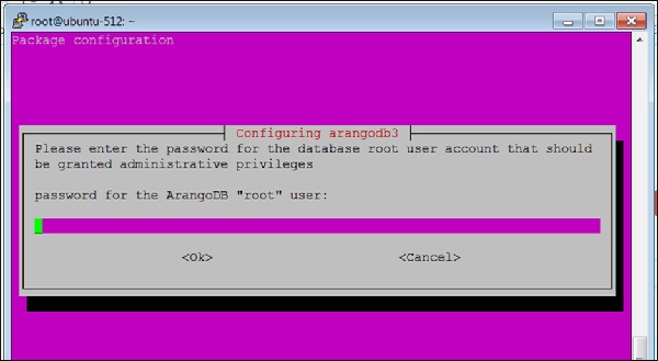
Here, you will be asked to provide a password for the ArangoDB root user. Note it down carefully.
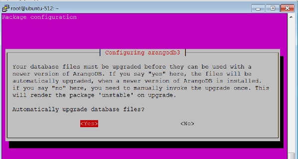
Select the yes option when the following dialog box appears −
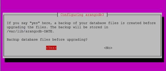
When you click Yes as in the above dialog box, the following dialog box appears. Click Yes here.
You can also check the status of ArangoDB with the following command −
# sudo systemctl status arangodb3
Output
arangodb3.service - LSB: arangodb
Loaded: loaded (/etc/init.d/arangodb3; bad; vendor pre set: enabled)
Active: active (running) since Mon 2017-09-04 05:42:35 UTC;
4min 46s ago
Docs: man:systemd-sysv-generator(8)
Process: 2642 ExecStart=/etc/init.d/arangodb3 start (code = exited,
status = 0/SUC
Tasks: 22
Memory: 158.6M
CPU: 3.117s
CGroup: /system.slice/arangodb3.service
├─2689 /usr/sbin/arangod --uid arangodb
--gid arangodb --pid-file /va
└─2690 /usr/sbin/arangod --uid arangodb
--gid arangodb --pid-file /va
Sep 04 05:42:33 ubuntu-512 systemd[1]: Starting LSB: arangodb...
Sep 04 05:42:33 ubuntu-512 arangodb3[2642]: * Starting arango database server a
Sep 04 05:42:35 ubuntu-512 arangodb3[2642]: {startup} starting up in daemon mode
Sep 04 05:42:35 ubuntu-512 arangodb3[2642]: changed working directory for child
Sep 04 05:42:35 ubuntu-512 arangodb3[2642]: ...done.
Sep 04 05:42:35 ubuntu-512 systemd[1]: StartedLSB: arang odb.
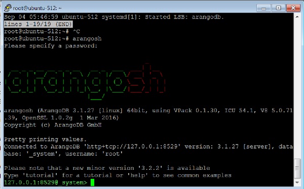
Sep 04 05:46:59 ubuntu-512 systemd[1]: Started LSB: arangodb. lines 1-19/19 (END)
ArangoDB is now ready to be used.
To invoke the arangosh terminal, type the following command in the terminal −
# arangosh
Output
Please specify a password:
Supply the root password created at the time of installation −
_
__ _ _ __ __ _ _ __ __ _ ___ | |
/ | ''__/ _ | ’ / ` |/ _ / | ’
| (| | | | (| | | | | (| | () _ | | |
_,|| _,|| ||_, |_/|/| ||
|__/
arangosh (ArangoDB 3.1.27 [linux] 64bit, using VPack 0.1.30, ICU 54.1, V8
5.0.71.39, OpenSSL 1.0.2g 1 Mar 2016)
Copyright (c) ArangoDB GmbH
Pretty printing values.
Connected to ArangoDB ''http+tcp://127.0.0.1:8529'' version: 3.1.27 [server],
database: ''_system'', username: ''root''
Please note that a new minor version ''3.2.2'' is available
Type ''tutorial'' for a tutorial or ''help'' to see common examples
127.0.0.1:8529@_system> exit
To log out from ArangoDB, type the following command −
127.0.0.1:8529@_system> exit
Output
Uf wiederluege! Na shledanou! Auf Wiedersehen! Bye Bye! Adiau! ¡Hasta luego!
Εις το επανιδείν!
להתראות ! Arrivederci! Tot ziens! Adjö! Au revoir! さようなら До свидания! Até
Breve! !خداحافظ
ArangoDB – Command Line
In this chapter, we will discuss how Arangosh works as the Command Line for ArangoDB. We will start by learning how to add a Database user.
Note − Remember numeric keypad might not work on Arangosh.
Let us assume that the user is “harry” and password is “hpwdb”.
127.0.0.1:8529@_system> require("org/arangodb/users").save("harry", "hpwdb");
Output
{
"user" : "harry",
"active" : true,
"extra" : {},
"changePassword" : false,
"code" : 201
}
ArangoDB – Web Interface
In this chapter, we will learn how to enable/disable the Authentication, and how to bind the ArangoDB to the Public Network Interface.
# arangosh --server.endpoint tcp://127.0.0.1:8529 --server.database "_system"
It will prompt you for the password saved earlier −
Please specify a password:
Use the password you created for root, at the configuration.
You can also use curl to check that you are actually getting HTTP 401 (Unauthorized) server responses for requests that require authentication −
# curl --dump - http://127.0.0.1:8529/_api/version
Output
HTTP/1.1 401 Unauthorized
X-Content-Type-Options: nosniff
Www-Authenticate: Bearer token_type = "JWT", realm = "ArangoDB"
Server: ArangoDB
Connection: Keep-Alive
Content-Type: text/plain; charset = utf-8
Content-Length: 0
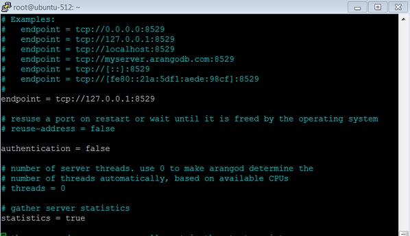
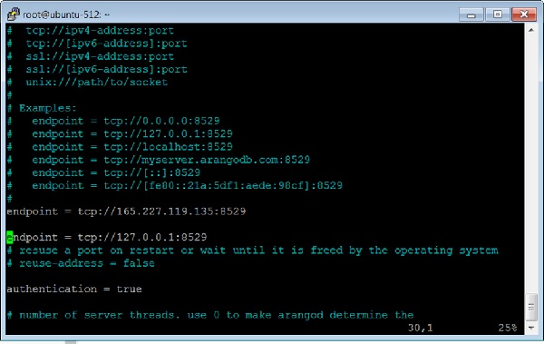
To avoid entering the password each time during our learning process, we will disable the authentication. For that, open the configuration file −
# vim /etc/arangodb3/arangod.conf
You should change the color scheme if the code is not properly visible.
:colorscheme desert
Set authentication to false as shown in the screenshot below.
Restart the service −
# service arangodb3 restart
On making the authentication false, you will be able to login (either with root or created user like Harry in this case) without entering any password in please specify a password.
Let us check the api version when the authentication is switched off −
# curl --dump - http://127.0.0.1:8529/_api/version
Output
HTTP/1.1 200 OK
X-Content-Type-Options: nosniff
Server: ArangoDB
Connection: Keep-Alive
Content-Type: application/json; charset=utf-8
Content-Length: 60
{"server":"arango","version":"3.1.27","license":"community"}
ArangoDB – Example Case Scenarios
In this chapter, we will consider two example scenarios. These examples are easier to comprehend and will help us understand the way the ArangoDB functionality works.
To demonstrate the APIs, ArangoDB comes preloaded with a set of easily understandable graphs. There are two methods to create instances of these graphs in your ArangoDB −
- Add Example tab in the create graph window in the web interface,
- or load the module @arangodb/graph-examples/example-graph in Arangosh.
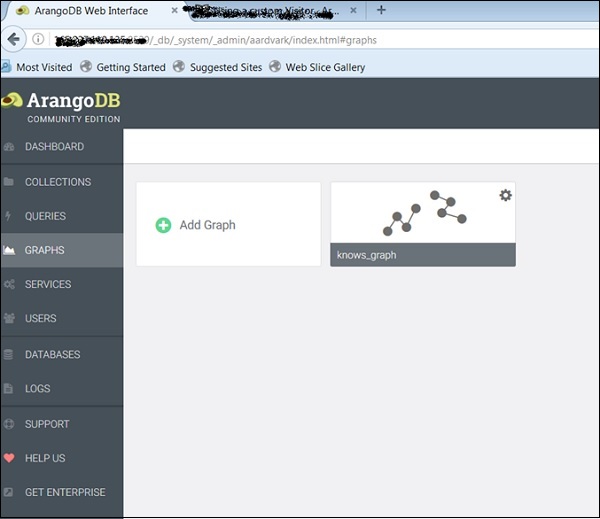
To start with, let us load a graph with the help of web interface. For that, launch the web interface and click on the graphs tab.
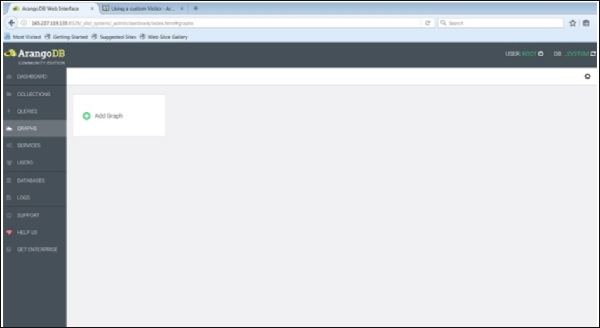
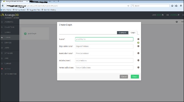
The Create Graph dialog box appears. The Wizard contains two tabs – Examples and Graph. The Graph tab is open by default; supposing we want to create a new graph, it will ask for the name and other definitions for the graph.
Now, we will upload the already created graph. For this, we will select the Examples tab.
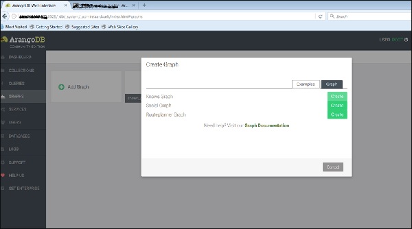
We can see the three example graphs. Select the Knows_Graph and click on the green button Create.
Once you have created them, you can inspect them in the web interface – which was used to create the pictures below.
The Knows_Graph
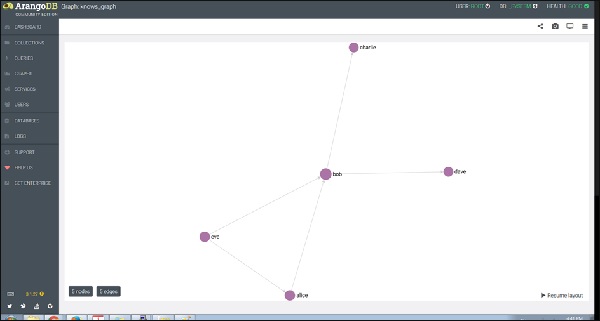
Let us now see how the Knows_Graph works. Select the Knows_Graph, and it will fetch the graph data.
The Knows_Graph consists of one vertex collection persons connected via one edge collection knows. It will contain five persons Alice, Bob, Charlie, Dave and Eve as vertices. We will have the following directed relations
Alice knows Bob
Bob knows Charlie
Bob knows Dave
Eve knows Alice
Eve knows Bob
If you click a node (vertex), say ‘bob’, it will show the ID (persons/bob) attribute name.
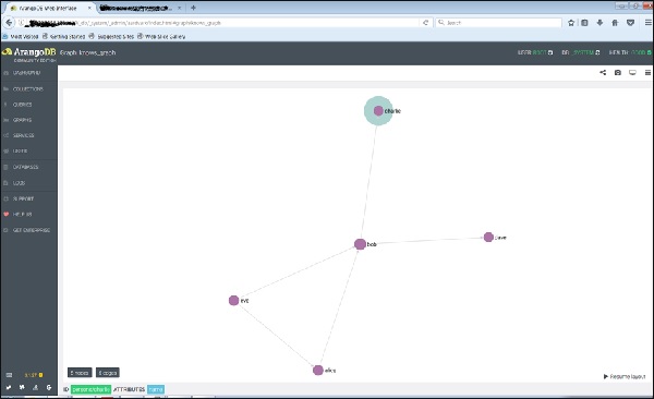
And on clicking any of the edge, it will show the ID (knows/4590) attributes.
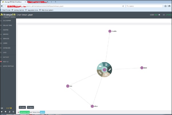
This is how we create it, inspect its vertices and edges.
Let us add another graph, this time using Arangosh. For that, we need to include another endpoint in the ArangoDB configuration file.
How to Add Multiple Endpoints
Open the configuration file −
# vim /etc/arangodb3/arangod.conf
Add another endpoint as shown in the terminal screenshot below.
Restart the ArangoDB −
# service arangodb3 restart
Launch the Arangosh −
# arangosh
Please specify a password:
_
__ _ _ __ __ _ _ __ __ _ ___ ___| |__
/ _` | ''__/ _` | ''_ / _` |/ _ / __| ''_
| (_| | | | (_| | | | | (_| | (_) __ | | |
__,_|_| __,_|_| |_|__, |___/|___/_| |_|
|___/
arangosh (ArangoDB 3.1.27 [linux] 64bit, using VPack 0.1.30, ICU 54.1, V8
5.0.71.39, OpenSSL 1.0.2g 1 Mar 2016)
Copyright (c) ArangoDB GmbH
Pretty printing values.
Connected to ArangoDB ''http+tcp://127.0.0.1:8529'' version: 3.1.27
[server], database: ''_system'', username: ''root''
Please note that a new minor version ''3.2.2'' is available
Type ''tutorial'' for a tutorial or ''help'' to see common examples
127.0.0.1:8529@_system>
The Social_Graph
Let us now understand what a Social_Graph is and how it works. The graph shows a set of persons and their relations −
This example has female and male persons as vertices in two vertex collections – female and male. The edges are their connections in the relation edge collection. We have described how to create this graph using Arangosh. The reader can work around it and explore its attributes, as we did with the Knows_Graph.
ArangoDB – Data Models and Modeling
In this chapter, we will focus on the following topics −
- Database Interaction
- Data Model
- Data Retrieval
ArangoDB supports document based data model as well as graph based data model. Let us first describe the document based data model.
ArangoDB”s documents closely resemble the JSON format. Zero or more attributes are contained in a document, and a value attached with each attribute. A value is either of an atomic type, such as a number, Boolean or null, literal string, or of a compound data type, such as embedded document/object or an array. Arrays or sub-objects may consist of these data types, which implies that a single document can represent non-trivial data structures.
Further in hierarchy, documents are arranged into collections, which may contain no documents (in theory) or more than one document. One can compare documents to rows and collections to tables (Here tables and rows refer to those of relational database management systems – RDBMS).
But, in RDBMS, defining columns is a prerequisite to store records into a table, calling these definitions schemas. However, as a novel feature, ArangoDB is schema-less – there is no a priori reason to specify what attributes the document will have.
And unlike RDBMS, each document can be structured in a completely different way from another document. These documents can be saved together in one single collection. Practically, common characteristics may exist among documents in the collection, however the database system, i.e., ArangoDB itself, does not bind you to a particular data structure.
Now we will try to understand ArangoDB”s [graph data model], which requires two kinds of collections — the first is the document collections (known as vertices collections in group-theoretic language), the second is the edge collections. There is a subtle difference between these two types. Edge collections also store documents, but they are characterized by including two unique attributes, _from and _to for creating relations between documents. In practice, a document (read edge) links two documents (read vertices), both stored in their respective collections. This architecture is derived from the graph-theoretic concept of a labeled, directed graph, excluding edges that can have not only labels, but can be a complete JSON like document in itself.
To compute fresh data, delete documents or to manipulate them, queries are used, which select or filter documents as per the given criteria. Either being simple as an “example query” or being as complex as “joins”, queries are coded in AQL – ArangoDB Query Language.
ArangoDB – Database Methods
In this chapter, we will discuss the different Database Methods in ArangoDB.
To start with, let us get the properties of the Database −
First, we invoke the Arangosh. Once, Arangosh is invoked, we will list the databases we created so far −
We will use the following line of code to invoke Arangosh −
127.0.0.1:8529@_system> db._databases()
Output
[
"_system",
"song_collection"
]
We see two databases, one _system created by default, and the second song_collection that we have created.
Let us now shift to song_collection database with the following line of code −
127.0.0.1:8529@_system> db._useDatabase("song_collection")
Output
true
127.0.0.1:8529@song_collection>
We will explore the properties of our song_collection database.
To find the name
We will use the following line of code to find the name.
127.0.0.1:8529@song_collection> db._name()
Output
song_collection
To find the id −
We will use the following line of code to find the id.
127.0.0.1:8529@song_collection> db._id()
Output
4838
To find the path −
We will use the following line of code to find the path.
127.0.0.1:8529@song_collection> db._path()
Output
/var/lib/arangodb3/databases/database-4838
Let us now check if we are in the system database or not by using the following line of
code −
127.0.0.1:8529@song_collection&t; db._isSystem()
Output
false
It means we are not in the system database (as we have created and shifted to the song_collection). The following screenshot will help you understand this.
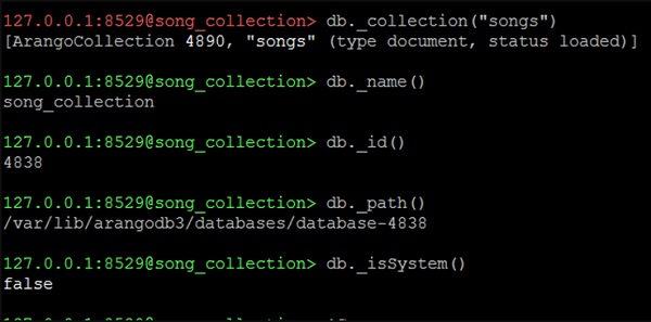
To get a particular collection, say songs −
We will use the following line of code the get a particular collection.
127.0.0.1:8529@song_collection> db._collection("songs")
Output
[ArangoCollection 4890, "songs" (type document, status loaded)]
The line of code returns a single collection.
Let us move to the essentials of the database operations with our subsequent chapters.
ArangoDB – Crud Operations
In this chapter, we will learn the different operations with Arangosh.
The following are the possible operations with Arangosh −
- Creating a Document Collection
- Creating Documents
- Reading Documents
- Updating Documents
Let us start by creating a new database. We will use the following line of code to create a new database −
127.0.0.1:8529@_system> db._createDatabase("song_collection")
true
The following line of code will help you shift to the new database −
127.0.0.1:8529@_system> db._useDatabase("song_collection")
true
Prompt will shift to “@@song_collection”
127.0.0.1:8529@song_collection>
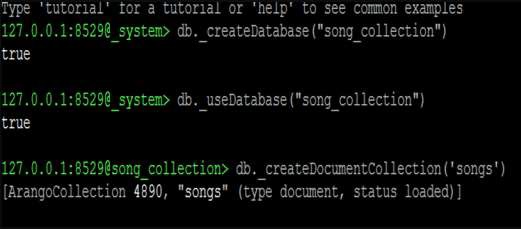
From here we will study CRUD Operations. Let us create a collection into the new database −
127.0.0.1:8529@song_collection> db._createDocumentCollection(''songs'')
Output
[ArangoCollection 4890, "songs" (type document, status loaded)]
127.0.0.1:8529@song_collection>
Let us add a few documents (JSON objects) to our ”songs” collection.
We add the first document in the following way −
127.0.0.1:8529@song_collection> db.songs.save({title: "A Man''s Best Friend",
lyricist: "Johnny Mercer", composer: "Johnny Mercer", Year: 1950, _key:
"A_Man"})
Output
{
"_id" : "songs/A_Man",
"_key" : "A_Man",
"_rev" : "_VjVClbW---"
}
Let us add other documents to the database. This will help us learn the process of querying the data. You can copy these codes and paste the same in Arangosh to emulate the process −
127.0.0.1:8529@song_collection> db.songs.save(
{
title: "Accentchuate The Politics",
lyricist: "Johnny Mercer",
composer: "Harold Arlen", Year: 1944,
_key: "Accentchuate_The"
}
)
{
"_id" : "songs/Accentchuate_The",
"_key" : "Accentchuate_The",
"_rev" : "_VjVDnzO---"
}
127.0.0.1:8529@song_collection> db.songs.save(
{
title: "Affable Balding Me",
lyricist: "Johnny Mercer",
composer: "Robert Emmett Dolan",
Year: 1950,
_key: "Affable_Balding"
}
)
{
"_id" : "songs/Affable_Balding",
"_key" : "Affable_Balding",
"_rev" : "_VjVEFMm---"
}
How to Read Documents
The _key or the document handle can be used to retrieve a document. Use document handle if there is no need to traverse the collection itself. If you have a collection, the document function is easy to use −
127.0.0.1:8529@song_collection> db.songs.document("A_Man");
{
"_key" : "A_Man",
"_id" : "songs/A_Man",
"_rev" : "_VjVClbW---",
"title" : "A Man''s Best Friend",
"lyricist" : "Johnny Mercer",
"composer" : "Johnny Mercer",
"Year" : 1950
}
How to Update Documents
Two options are available to update the saved data − replace and update.
The update function patches a document, merging it with the given attributes. On the other hand, the replace function will replace the previous document with a new one. The replacement will still occur even if completely different attributes are provided. We will first observe a non-destructive update, updating the attribute Production` in a song −
127.0.0.1:8529@song_collection> db.songs.update("songs/A_Man",{production:
"Top Banana"});
Output
{
"_id" : "songs/A_Man",
"_key" : "A_Man",
"_rev" : "_VjVOcqe---",
"_oldRev" : "_VjVClbW---"
}
Let us now read the updated song”s attributes −
127.0.0.1:8529@song_collection> db.songs.document(''A_Man'');
Output
{
"_key" : "A_Man",
"_id" : "songs/A_Man",
"_rev" : "_VjVOcqe---",
"title" : "A Man''s Best Friend",
"lyricist" : "Johnny Mercer",
"composer" : "Johnny Mercer",
"Year" : 1950,
"production" : "Top Banana"
}
A large document can be easily updated with the update function, especially when the attributes are very few.
In contrast, the replace function will abolish your data on using it with the same document.
127.0.0.1:8529@song_collection> db.songs.replace("songs/A_Man",{production:
"Top Banana"});
Let us now check the song we have just updated with the following line of code −
127.0.0.1:8529@song_collection> db.songs.document(''A_Man'');
Output
{
"_key" : "A_Man",
"_id" : "songs/A_Man",
"_rev" : "_VjVRhOq---",
"production" : "Top Banana"
}
Now, you can observe that the document no longer has the original data.
How to Remove Documents
The remove function is used in combination with the document handle to remove a document from a collection −
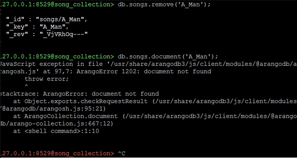
127.0.0.1:8529@song_collection> db.songs.remove(''A_Man'');
Let us now check the song”s attributes we just removed by using the following line of code −
127.0.0.1:8529@song_collection> db.songs.document(''A_Man'');
We will get an exception error like the following as an output −
JavaScript exception in file
''/usr/share/arangodb3/js/client/modules/@arangodb/arangosh.js'' at 97,7:
ArangoError 1202: document not found
! throw error;
! ^
stacktrace: ArangoError: document not found
at Object.exports.checkRequestResult
(/usr/share/arangodb3/js/client/modules/@arangodb/arangosh.js:95:21)
at ArangoCollection.document
(/usr/share/arangodb3/js/client/modules/@arangodb/arango-collection.js:667:12)
at <shell command>:1:10
Crud Operations using Web Interface
In our previous chapter, we learned how to perform various operations on documents with Arangosh, the command line. We will now learn how to perform the same operations using the web interface. To start with, put the following address – http://your_server_ip:8529/_db/song_collection/_admin/aardvark/index.html#login in the address bar of your browser. You will be directed to the following login page.
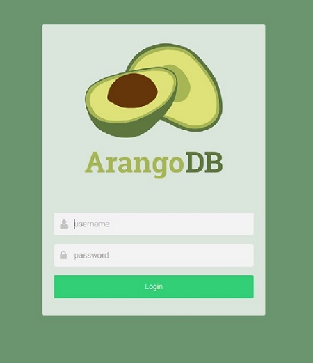
Now, enter the username and password.
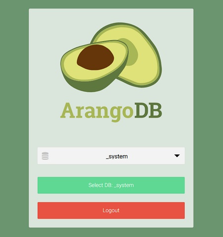
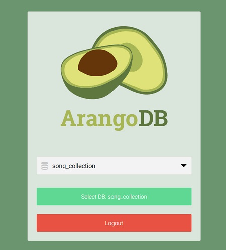
If it is successful, the following screen appears. We need to make a choice for the database to work on, the _system database being the default one. Let us choose the song_collection database, and click on the green tab −
Creating a Collection
In this section, we will learn how to create a collection. Press the Collections tab in the navigation bar at the top.
Our command line added songs collection are visible. Clicking on that will show the entries. We will now add an artists’ collection using the web interface. Collection songs which we created with Arangosh is already there. In the Name field, write artists in the New Collection dialog box that appears. Advanced options can safely be ignored and the default collection type, i.e. Document, is fine.
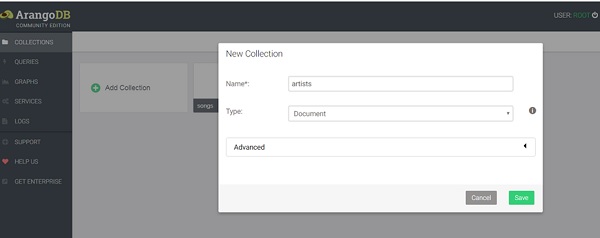
Clicking on the Save button will finally create the collection, and now the two collections will be visible on this page.
Filling Up the Newly Created Collection with Documents
You will be presented with an empty collection on clicking the artists collection −
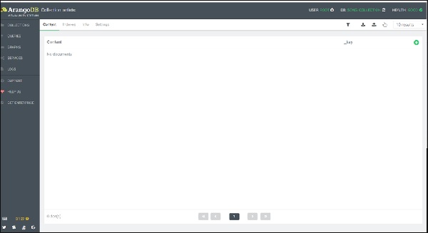
To add a document, you need to click the + sign placed in the upper right corner. When you are prompted for a _key, enter Affable_Balding as the key.
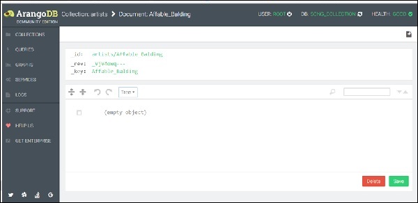
Now, a form will appear to add and edit the attributes of the document. There are two ways of adding attributes: Graphical and Tree. The graphical way is intuitive but slow, therefore, we will switch to the Code view, using the Tree dropdown menu to select it −
To make the process easier, we have created a sample data in the JSON format, which you can copy and then paste into the query editor area −
{“artist”: “Johnny Mercer”, “title”:”Affable Balding Me”, “composer”: “Robert Emmett
Dolan”, “Year”: 1950}
(Note: Only one pair of curly braces should be used; see the screenshot below)
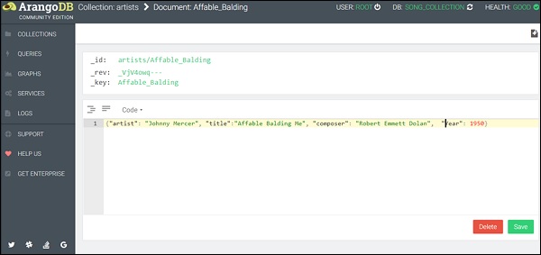
You can observe that we have quoted the keys and also the values in the code view mode. Now, click Save. Upon successful completion, a green flash appears on the page momentarily.
How to Read Documents
To read documents, go back to the Collections page.
When one clicks on the artist collection, a new entry appears.
How to Update Documents
It is simple to edit the entries in a document; you just need to click on the row you wish to edit in the document overview. Here again the same query editor will be presented as when creating new documents.
Removing Documents
You can delete the documents by pressing the ‘-’ icon. Every document row has this sign at the end. It will prompt you to confirm to avoid unsafe deletion.
Moreover, for a particular collection, other operations like filtering the documents, managing indexes, and importing data also exist on the Collections Overview page.
In our subsequent chapter, we will discuss an important feature of the Web Interface, i.e., the AQL query Editor.
Querying the Data with AQL
In this chapter, we will discuss how to query the data with AQL. We have already discussed in our previous chapters that ArangoDB has developed its own query language and that it goes by the name AQL.
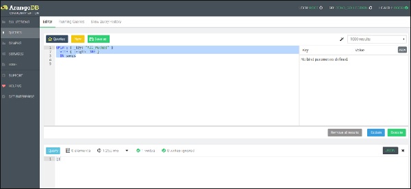
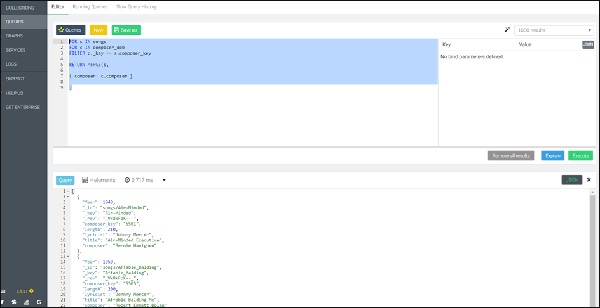
Let us now start interacting with AQL. As shown in the image below, in the web interface, press the AQL Editor tab placed at the top of the navigation bar. A blank query editor will appear.
When need, you can switch to the editor from the result view and vice-versa, by clicking the Query or the Result tabs in the top right corner as shown in the image below −
Among other things, the editor has syntax highlighting, undo/redo functionality, and query saving. For a detailed reference, one can see the official documentation. We will highlight few basic and commonly-used features of the AQL query editor.
AQL Fundamentals
In AQL, a query represents the end result to be achieved, but not the process through which the end result is to be achieved. This feature is commonly known as a declarative property of the language. Moreover, AQL can query as well modify the data, and thus complex queries can be created by combining both the processes.
Please note that AQL is entirely ACID-compliant. Reading or modifying queries will either conclude in whole or not at all. Even reading a document”s data will finish with a consistent unit of the data.
We add two new songs to the songs collection we have already created. Instead of typing, you can copy the following query, and paste it in the AQL editor −
FOR song IN [
   {
      title: "Air-Minded Executive", lyricist: "Johnny Mercer",
      composer: "Bernie Hanighen", Year: 1940, _key: "Air-Minded"
   },

   {
      title: "All Mucked Up", lyricist: "Johnny Mercer", composer:
      "Andre Previn", Year: 1974, _key: "All_Mucked"
   }
]
INSERT song IN songs
Press the Execute button at the lower left.
It will write two new documents in the songs collection.
This query describes how the FOR loop works in AQL; it iterates over the list of JSON encoded documents, performing the coded operations on each one of the documents in the collection. The different operations can be creating new structures, filtering, selecting documents, modifying, or inserting documents into the database (refer the instantaneous example). In essence, AQL can perform the CRUD operations efficiently.
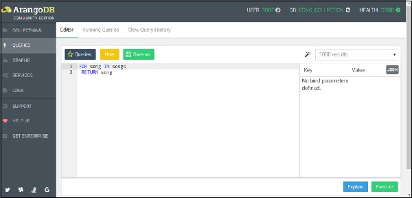
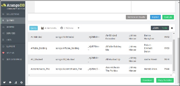
To find all the songs in our database, let us once again run the following query, equivalent to a SELECT * FROM songs of an SQL-type database (because the editor memorizes the last query, press the *New* button to clean the editor) −
FOR song IN songs
RETURN song
The result set will show the list of songs so far saved in the songs collection as shown in the screenshot below.
Operations like FILTER, SORT and LIMIT can be added to the For loop body to narrow and order the result.
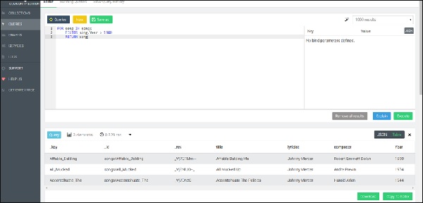
FOR song IN songs
FILTER song.Year > 1940
RETURN song
The above query will give songs created after the year 1940 in the Result tab (see the image below).
The document key is used in this example, but any other attribute can also be used as an equivalent for filtering. Since the document key is guaranteed to be unique, no more than a single document will match this filter. For other attributes this may not be the case. To return a subset of active users (determined by an attribute called status), sorted by name in ascending order, we use the following syntax −
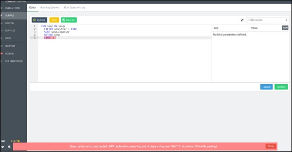
FOR song IN songs
FILTER song.Year > 1940
SORT song.composer
RETURN song
LIMIT 2
We have deliberately included this example. Here, we observe a query syntax error message highlighted in red by AQL. This syntax highlights the errors and is helpful in debugging your queries as shown in the screenshot below.
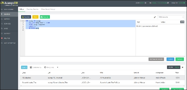
Let us now run the correct query (note the correction) −
FOR song IN songs
FILTER song.Year > 1940
SORT song.composer
LIMIT 2
RETURN song
Complex Query in AQL
AQL is equipped with multiple functions for all supported data types. Variable assignment within a query allows to build very complex nested constructs. This way data-intensive operations move closer to the data at the backend than on to the client (such as browser). To understand this, let us first add the arbitrary durations (length) to songs.
Let us start with the first function, i.e., the Update function −
UPDATE { _key: "All_Mucked" }
WITH { length: 180 }
IN songs
We can see one document has been written as shown in the above screenshot.
Let us now update other documents (songs) too.
UPDATE { _key: "Affable_Balding" }
WITH { length: 200 }
IN songs
We can now check that all our songs have a new attribute length −
FOR song IN songs
RETURN song
Output
[
   {
      "_key": "Air-Minded",
      "_id": "songs/Air-Minded",
      "_rev": "_VkC5lbS---",
      "title": "Air-Minded Executive",
      "lyricist": "Johnny Mercer",
      "composer": "Bernie Hanighen",
      "Year": 1940,
      "length": 210
   },

   {
      "_key": "Affable_Balding",
      "_id": "songs/Affable_Balding",
      "_rev": "_VkC4eM2---",
      "title": "Affable Balding Me",
      "lyricist": "Johnny Mercer",
      "composer": "Robert Emmett Dolan",
      "Year": 1950,
      "length": 200
   },

   {
      "_key": "All_Mucked",
      "_id": "songs/All_Mucked",
      "_rev": "_Vjah9Pu---",
      "title": "All Mucked Up",
      "lyricist": "Johnny Mercer",
      "composer": "Andre Previn",
      "Year": 1974,
      "length": 180
   },

   {
      "_key": "Accentchuate_The",
      "_id": "songs/Accentchuate_The",
      "_rev": "_VkC3WzW---",
      "title": "Accentchuate The Politics",
      "lyricist": "Johnny Mercer",
      "composer": "Harold Arlen",
      "Year": 1944,
      "length": 190
   }
]
To illustrate the use of other keywords of AQL such as LET, FILTER, SORT, etc., we now format the song”s durations in the mm:ss format.
Query
FOR song IN songs
FILTER song.length > 150
LET seconds = song.length % 60
LET minutes = FLOOR(song.length / 60)
SORT song.composer
RETURN
{
   Title: song.title,
   Composer: song.composer,
   Duration: CONCAT_SEPARATOR('':'',minutes, seconds)
}
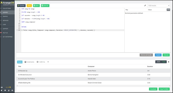
This time we will return the song title together with the duration. The Return function lets you create a new JSON object to return for each input document.
We will now talk about the ‘Joins’ feature of AQL database.
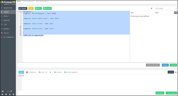
Let us begin by creating a collection composer_dob. Further, we will create the four documents with the hypothetical date of births of the composers by running the following query in the query box −
FOR dob IN [
   {composer: "Bernie Hanighen", Year: 1909}
   ,
   {composer: "Robert Emmett Dolan", Year: 1922}
   ,
   {composer: "Andre Previn", Year: 1943}
   ,
   {composer: "Harold Arlen", Year: 1910}
]
INSERT dob in composer_dob
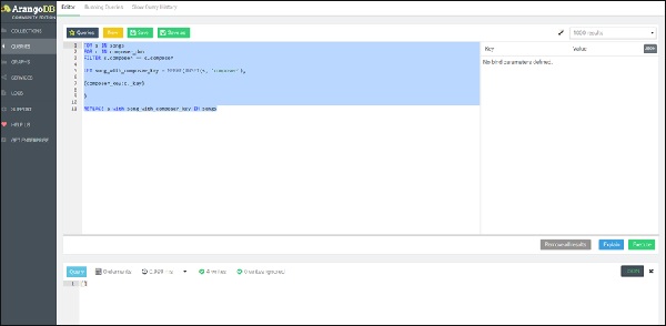
To highlight the similarity with SQL, we present a nested FOR-loop query in AQL, leading to the REPLACE operation, iterating first in the inner loop, over all the composers’ dob and then on all the associated songs, creating a new document containing attribute song_with_composer_key instead of the song attribute.
Here goes the query −
FOR s IN songs
FOR c IN composer_dob
FILTER s.composer == c.composer

LET song_with_composer_key = MERGE(
   UNSET(s, ''composer''),
   {composer_key:c._key}
)
REPLACE s with song_with_composer_key IN songs
Let us now run the query FOR song IN songs RETURN song again to see how the song collection has changed.
Output
[
   {
      "_key": "Air-Minded",
      "_id": "songs/Air-Minded",
      "_rev": "_Vk8kFoK---",
      "Year": 1940,
      "composer_key": "5501",
      "length": 210,
      "lyricist": "Johnny Mercer",
      "title": "Air-Minded Executive"
   },

   {
      "_key": "Affable_Balding",
      "_id": "songs/Affable_Balding",
      "_rev": "_Vk8kFoK--_",
      "Year": 1950,
      "composer_key": "5505",
      "length": 200,
      "lyricist": "Johnny Mercer",
      "title": "Affable Balding Me"
   },

   {
      "_key": "All_Mucked",
      "_id": "songs/All_Mucked",
      "_rev": "_Vk8kFoK--A",
      "Year": 1974,
      "composer_key": "5507",
      "length": 180,
      "lyricist": "Johnny Mercer",
      "title": "All Mucked Up"
   },

   {
      "_key": "Accentchuate_The",
      "_id": "songs/Accentchuate_The",
      "_rev": "_Vk8kFoK--B",
      "Year": 1944,
      "composer_key": "5509",
      "length": 190,
      "lyricist": "Johnny Mercer",
      "title": "Accentchuate The Politics"
   }
]
The above query completes the data migration process, adding the composer_key to each song.
Now the next query is again a nested FOR-loop query, but this time leading to the Join operation, adding the associated composer”s name (picking with the help of `composer_key`) to each song −
FOR s IN songs
FOR c IN composer_dob
FILTER c._key == s.composer_key
RETURN MERGE(s,
{ composer: c.composer }
)
Output
[
   {
      "Year": 1940,
      "_id": "songs/Air-Minded",
      "_key": "Air-Minded",
      "_rev": "_Vk8kFoK---",
      "composer_key": "5501",
      "length": 210,
      "lyricist": "Johnny Mercer",
      "title": "Air-Minded Executive",
      "composer": "Bernie Hanighen"
   },

   {
      "Year": 1950,
      "_id": "songs/Affable_Balding",
      "_key": "Affable_Balding",
      "_rev": "_Vk8kFoK--_",
      "composer_key": "5505",
      "length": 200,
      "lyricist": "Johnny Mercer",
      "title": "Affable Balding Me",
      "composer": "Robert Emmett Dolan"
   },

   {
      "Year": 1974,
      "_id": "songs/All_Mucked",
      "_key": "All_Mucked",
      "_rev": "_Vk8kFoK--A",
      "composer_key": "5507",
      "length": 180,
      "lyricist": "Johnny Mercer",
      "title": "All Mucked Up",
      "composer": "Andre Previn"
   },

   {
      "Year": 1944,
      "_id": "songs/Accentchuate_The",
      "_key": "Accentchuate_The",
      "_rev": "_Vk8kFoK--B",
      "composer_key": "5509",
      "length": 190,
      "lyricist": "Johnny Mercer",
      "title": "Accentchuate The Politics",
      "composer": "Harold Arlen"
   }
]
ArangoDB – AQL Example Queries
In this chapter, we will consider a few AQL Example Queries on an Actors and Movies Database. These queries are based on graphs.
Problem
Given a collection of actors and a collection of movies, and an actIn edges collection (with a year property) to connect the vertex as indicated below −
[Actor] <- act in -> [Movie]
How do we get −
- All actors who acted in “movie1” OR “movie2”?
- All actors who acted in both “movie1” AND “movie2”?
- All common movies between “actor1” and “actor2”?
- All actors who acted in 3 or more movies?
- All movies where exactly 6 actors acted in?
- The number of actors by movie?
- The number of movies by actor?
- The number of movies acted in between 2005 and 2010 by actor?
Solution
During the process of solving and obtaining the answers to the above queries, we will use Arangosh to create the dataset and run queries on that. All the AQL queries are strings and can simply be copied over to your favorite driver instead of Arangosh.
Let us start by creating a Test Dataset in Arangosh. First, download −
# wget -O dataset.js
Output
...
HTTP request sent, awaiting response... 200 OK
Length: unspecified [text/html]
Saving to: ‘dataset.js’
dataset.js [ <=> ] 115.14K --.-KB/s in 0.01s
2017-09-17 14:19:12 (11.1 MB/s) - ‘dataset.js’ saved [117907]
You can see in the output above that we have downloaded a JavaScript file dataset.js. This file contains the Arangosh commands to create the dataset in the database. Instead of copying and pasting the commands one by one, we will use the –javascript.execute option on Arangosh to execute the multiple commands non-interactively. Consider it the life saver command!
Now execute the following command on the shell −
$ arangosh --javascript.execute dataset.js
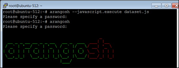
Supply the password when prompted as you can see in the above screenshot. Now we have saved the data, so we will construct the AQL queries to answer the specific questions raised in the beginning of this chapter.
First Question
Let us take the first question: All actors who acted in “movie1” OR “movie2”. Suppose, we want to find the names of all the actors who acted in “TheMatrix” OR “TheDevilsAdvocate” −
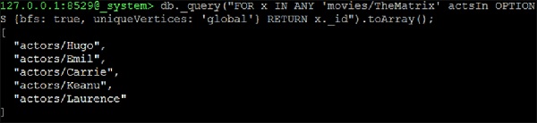
We will start with one movie at a time to get the names of the actors −
127.0.0.1:8529@_system> db._query("FOR x IN ANY ''movies/TheMatrix'' actsIn
OPTIONS {bfs: true, uniqueVertices: ''global''} RETURN x._id").toArray();
Output
We will receive the following output −
[
   "actors/Hugo",
   "actors/Emil",
   "actors/Carrie",
   "actors/Keanu",
   "actors/Laurence"
]
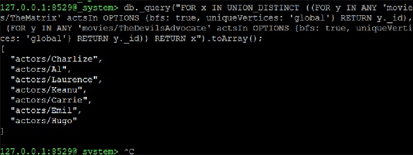
Now we continue to form a UNION_DISTINCT of two NEIGHBORS queries which will be the solution −
127.0.0.1:8529@_system> db._query("FOR x IN UNION_DISTINCT ((FOR y IN ANY
''movies/TheMatrix'' actsIn OPTIONS {bfs: true, uniqueVertices: ''global''} RETURN
y._id), (FOR y IN ANY ''movies/TheDevilsAdvocate'' actsIn OPTIONS {bfs: true,
uniqueVertices: ''global''} RETURN y._id)) RETURN x").toArray();
Output
[
   "actors/Charlize",
   "actors/Al",
   "actors/Laurence",
   "actors/Keanu",
   "actors/Carrie",
   "actors/Emil",
   "actors/Hugo"
]
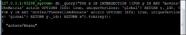
Second Question
Let us now consider the second question: All actors who acted in both “movie1” AND “movie2”. This is almost identical to the question above. But this time we are not interested in a UNION but in an INTERSECTION −
127.0.0.1:8529@_system> db._query("FOR x IN INTERSECTION ((FOR y IN ANY
''movies/TheMatrix'' actsIn OPTIONS {bfs: true, uniqueVertices: ''global''} RETURN
y._id), (FOR y IN ANY ''movies/TheDevilsAdvocate'' actsIn OPTIONS {bfs: true,
uniqueVertices: ''global''} RETURN y._id)) RETURN x").toArray();
Output
We will receive the following output −
[
   "actors/Keanu"
]
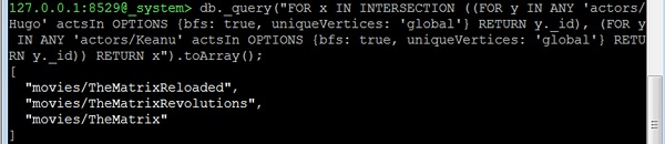
Third Question
Let us now consider the third question: All common movies between “actor1” and “actor2”. This is actually identical to the question about common actors in movie1 and movie2. We just have to change the starting vertices. As an example, let us find all the movies where Hugo Weaving (“Hugo”) and Keanu Reeves are co-starring −
127.0.0.1:8529@_system> db._query(
   "FOR x IN INTERSECTION (
      (
         FOR y IN ANY ''actors/Hugo'' actsIn OPTIONS
         {bfs: true, uniqueVertices: ''global''}
          RETURN y._id
      ),

      (
         FOR y IN ANY ''actors/Keanu'' actsIn OPTIONS
         {bfs: true, uniqueVertices:''global''} RETURN y._id
      )
   )
   RETURN x").toArray();
Output
We will receive the following output −
[
   "movies/TheMatrixReloaded",
   "movies/TheMatrixRevolutions",
   "movies/TheMatrix"
]
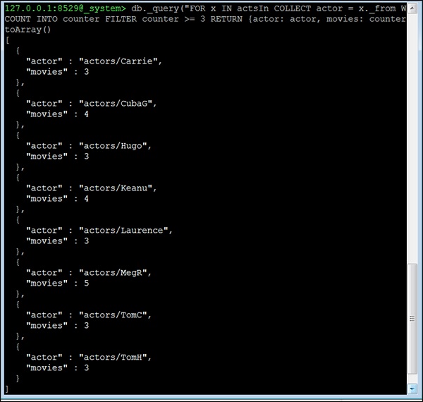
Fourth Question
Let us now consider the fourth question. All actors who acted in 3 or more movies. This question is different; we cannot make use of the neighbors function here. Instead we will make use of the edge-index and the COLLECT statement of AQL for grouping. The basic idea is to group all edges by their startVertex (which in this dataset is always the actor). Then we remove all actors with less than 3 movies from the result as here we have included the number of movies an actor has acted in −
127.0.0.1:8529@_system> db._query("FOR x IN actsIn COLLECT actor = x._from WITH
COUNT INTO counter FILTER counter >= 3 RETURN {actor: actor, movies:
counter}"). toArray()
Output
[
   {
      "actor" : "actors/Carrie",
      "movies" : 3
   },

   {
      "actor" : "actors/CubaG",
      "movies" : 4
   },

   {
      "actor" : "actors/Hugo",
      "movies" : 3
   },

   {
      "actor" : "actors/Keanu",
      "movies" : 4
   },

   {
      "actor" : "actors/Laurence",
      "movies" : 3
   },

   {
      "actor" : "actors/MegR",
      "movies" : 5
   },

   {
      "actor" : "actors/TomC",
      "movies" : 3
   },

   {
      "actor" : "actors/TomH",
      "movies" : 3
   }
]
For the remaining questions, we will discuss the query formation, and provide the queries only. The reader should run the query themselves on the Arangosh terminal.
Fifth Question
Let us now consider the fifth question: All movies where exactly 6 actors acted in. The same idea as in the query before, but with the equality filter. However, now we need the movie instead of the actor, so we return the _to attribute −
db._query("FOR x IN actsIn COLLECT movie = x._to WITH COUNT INTO counter FILTER
counter == 6 RETURN movie").toArray()
The number of actors by movie?
We remember in our dataset _to on the edge corresponds to the movie, so we count how
often the same _to appears. This is the number of actors. The query is almost identical to
the ones before but without the FILTER after COLLECT −
db._query("FOR x IN actsIn COLLECT movie = x._to WITH COUNT INTO counter RETURN
{movie: movie, actors: counter}").toArray()
Sixth Question
Let us now consider the sixth question: The number of movies by an actor.
The way we found solutions to our above queries will help you find the solution to this query as well.
db._query("FOR x IN actsIn COLLECT actor = x._from WITH COUNT INTO counter
RETURN {actor: actor, movies: counter}").toArray()
ArangoDB – How to Deploy
In this chapter, we will describe various possibilities to deploy ArangoDB.
Deployment: Single Instance
We have already learned how to deploy the single instance of the Linux (Ubuntu) in one of our previous chapters. Let us now see how to make the deployment using Docker.
Deployment: Docker
For deployment using docker, we will install Docker on our machine. For more information on Docker, please refer our tutorial on .
Once Docker is installed, you can use the following command −
docker run -e ARANGO_RANDOM_ROOT_PASSWORD = 1 -d --name agdb-foo -d
arangodb/arangodb
It will create and launch the Docker instance of ArangoDB with the identifying name agdbfoo as a Docker background process.
Also terminal will print the process identifier.
By default, port 8529 is reserved for ArangoDB to listen for requests. Also this port is automatically available to all Docker application containers which you may have linked.